www.geosci-model-dev.net/7/1175/2014/ doi:10.5194/gmd-7-1175-2014
© Author(s) 2014. CC Attribution 3.0 License.
Development of a tangent linear model (version 1.0) for the
High-Order Method Modeling Environment dynamical core
S. Kim, B.-J. Jung, and Y. Jo
Korea Institute of Atmospheric Prediction Systems, Seoul, South Korea Correspondence to: B.-J. Jung ([email protected])
Received: 7 January 2014 – Published in Geosci. Model Dev. Discuss.: 28 January 2014 Revised: 16 May 2014 – Accepted: 16 May 2014 – Published: 17 June 2014
Abstract. We describe development and validation of a tan-gent linear model for the High-Order Method Modeling En-vironment, the default dynamical core in the Community At-mosphere Model and the Community Earth System Model that solves a primitive hydrostatic equation using a spec-tral element method. A tangent linear model is primarily in-tended to approximate the evolution of perturbations gener-ated by a nonlinear model, provides a computationally ef-ficient way to calculate a nonlinear model trajectory for a short time range, and serves as an intermediate step to write and test adjoint models, as the forward model in the incre-mental approach to four-dimensional variational data assim-ilation, and as a tool for stability analysis. Each module in the tangent linear model (version 1.0) is linearized by hands-on derivatihands-ons, and is validated by the Taylor–Lagrange for-mula. The linearity checks confirm all modules correctly de-veloped, and the field results of the tangent linear modules converge to the difference field of two nonlinear modules as the magnitude of the initial perturbation is sequentially re-duced. Also, experiments for stable integration of the tangent linear model (version 1.0) show that the linear model is also suitable with an extended time step size compared to the time step of the nonlinear model without reducing spatial resolu-tion, or increasing further computational cost. Although the scope of the current implementation leaves room for a set of natural extensions, the results and diagnostic tools pre-sented here should provide guidance for further development of the next generation of the tangent linear model, the cor-responding adjoint model, and four-dimensional variational data assimilation, with respect to resolution changes and im-provements in linearized physics and dynamics.
1 Introduction
It has long been recognized that data assimilation (DA) schemes play a key role in numerical weather prediction (NWP) systems to correctly forecast short-range predictions. Among various DA schemes, four-dimensional variational DA (4DVar) methods have shown superior forecasting re-sults. In addition, a recent advent of fast multiprocessor com-puters leads the full potential of 4DVar to be realized in more complicated systems. 4DVar schemes including incre-mental 4DVar (Courtier et al., 1994), weak 4DVar (Yannick, 2007), and direct/indirect representative method (Bennett, 2002) generally all share the common components such as a tangent linear model (TLM), its adjoint model (ADM), a background error covariance, and minimization algorithms as 4DVar drivers.
For operational NWP applications, the construction of a TLM is a very important intermediate step in the develop-ment of the 4DVar. The TLM serves as an intermediate step to write and test the ADM, as the forward model in the incre-mental approach to 4DVar, and as a tool for stability analysis (Zhu and Kamachi, 2000; Ehrendorfer and Errico, 1995). It is essential for development of the 4DVar schemes to obtain consistency between the nonlinear model and its correspond-ing TLM that leads to the accurate development of its ADM, which plays a key role in finding a best initial condition by providing the gradient of the cost functional via minimiza-tion algorithms in the 4DVar schemes. Therefore, the TLMs have been recognized as powerful tools for analyzing numer-ous aspects such as model sensitivity and the dynamics of flow fields, and the evolution of perturbations.
1176 S. Kim et al.: Development of a tangent linear model (version 1.0)
here is the High-Order Method Modeling Environment (HOMME, www.homme.ucar.edu). The HOMME is a high-order method that utilizes fully unstructured quadrilateral-based finite element meshes on the sphere, and adopts a spec-tral element and discontinuous Galerkin method (Dennis et al., 2012). For its scalability and efficiency, the HOMME is considered as a promising dynamical core, and is the de-fault dynamical core of the Community Atmosphere Model (CAM) and the Community Earth System Model (CESM). Here, we developed a TLM for the HOMME dynamical core that can describe well the evolution of perturbations gener-ated by the nonlinear model when the magnitude of pertur-bation becomes the size of actual uncertainties (Errico and Raeder, 1999).
The second section explains the TLM development for the HOMME model including the description of the HOMME, time increment with management of temporal trajectories for the nonlinear model, and linearity checks. The third section shows the numerical results of the linearity checks for all tan-gent linear modules, including full fields for baroclinic insta-bilities of time-dependent zonal geostrophic flow, followed by a summary and discussion in the fourth section.
2 Development of tangent linear model
There are a couple of different ways to develop a TLM for a given dynamical model such as (1) a perturbation fore-casting approach in which the TLM is discretized from the linearization of the given nonlinear dynamical equation, and (2) a line-by-line approach in which the TLM is linearized directly from the numerical codes of the given dynamical model. The advantage of the former is that the approach can easily deal with numerical instability compared to the latter, but the TLM can be more conveniently developed by the lat-ter approach. Here, the line-by-line approach for the TLM development is adopted because of its straightforwardness of linearization for the set of the discretized nonlinear equa-tions. The complete source codes of the described modules are available from the authors upon request.
2.1 HOMME dynamical core
The HOMME is a high-order element-based method to build scalable, accurate, and conservative atmospheric general cir-culation models that numerically solves three-dimensional primitive equations (Nair and Tufo, 2007). HOMME em-ploys advanced time stepping, adaptive mesh refinement and several domain decomposition strategies along with the continuous/discontinuous Galerkin (CG/DG) and spec-tral element (SE) methods (Thomas and Loft, 2002; Dennis et al., 2012). Also, HOMME guarantees conservation and maintains all the attractive computational features of SE. Among the various horizontal discretization methods within
HOMME, the TLM development is targeted for CG method in this study.
The numerical configuration for HOMME and its TLM share the same numerical configuration. HOMME can be configured to solve the shallow water or the dry/moist prim-itive equations. The baroclinic test case (Jablonowski and Williamson, 2006) configured in HOMME is utilized to ap-praise the evolution of baroclinic waves in the Northern Hemisphere using quasi-realistic initial conditions, and em-ploys the second-order explicit Runge–Kutta time integra-tion. The computational domain is the global sphere that is covered by six identical regions by an equiangular central projection of the faces of an inscribed cube. Each face of the cubed sphere is free of singularities and is partitioned into
Ne byNe rectangular non-overlapping elements (so the to-tal number of elements is 6×Ne2). For each element of the computational domain, an approximate solution is expanded by a tensor product of Lagrange basis function of orderNp defined at the Gauss–Lobatto–Legendre (GLL) points. For this study, the conservative three-dimensional CG model is configured for the global sphere withNe=16,Np=4, and the horizontal resolution of 26 Lagrangian surfaces (i.e., the number of vertical levels Nlev=26). Then, the total num-ber of the elements isNelem=1536, and the grid resolution over the equatorial nodes is about 220 km, on average. A fourth-order hyperviscosity filter is used for spatial filtering, and the time increment is1t=150 s. Note that although the HOMME uses adaptive time stepping and adaptive mesh re-finement, its TLM does not include such functions. Message Passing Interface (MPI) domain decomposition through the space-filling curve approach is used for parallelism (Nair et al., 2009).
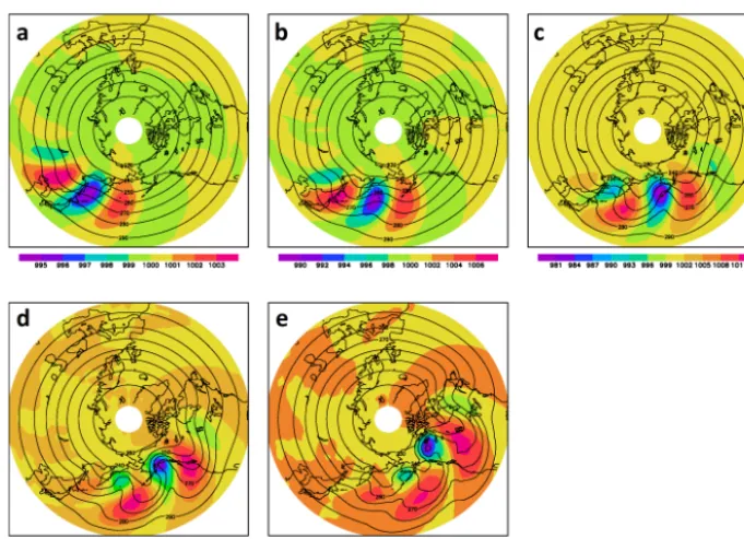
The evolution of the baroclinic wave is very slow from integration day 0 to day 4. Therefore, Fig. 1 only shows the triggering baroclinic waves and corresponding surface pressurePs and temperature fieldT at 850 hPa (Nlev=23) from day 6 to day 10. At days 6 and 7 the surface pressure shows few weak high- and low-pressure systems with shad-ings, and the temperature field exhibits the growth of very small-amplitude waves with contours (Fig. 1a, b). At day 8 the baroclinic instability waves are well developed in surface pressure, and the temperature waves are also clearly observed (Fig. 1c). The baroclinic pressure waves become strong at days 9 and 10, and the waves in the temperature field are almost peaked and begin to wrap around the trailing fronts (Fig. 1d, e).
2.2 Line-by-line approach
16 1
Figure 1.Evolution of the baroclinic wave from time integration with different days. The 2
shadings and contours represents surface pressure (hPa) and temperature (K), respectively. (a) 3
day 6, (b) 7, (c) 8, (d) 9, (e) 10. 4
5
Figure 1. Evolution of the baroclinic wave from time integration with different days. The shadings and contours represent surface pressure
(hPa) and temperature (K), respectively: (a) day 6, (b) 7, (c) 8, (d) 9, and (e) 10.
1. Determine input and output for variables and constants in the nonlinear codes.
2. Distinguish the variables for the tangent linear codes from those coefficients for nonlinear results by adding prefix “tl_”.
3. Linearize the nonlinear codes via the chain rule of the implicit derivative (or calculus of variation).
4. Check and clean up input and output variables in the module name.
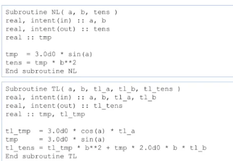
In Fig. 2, input and output for the variables in both nonlinear (NL) and tangent linear (TL) codes are indicated by intent(in) and intent(out). The variables for the NL code area,band tens, while the variables for the TL code are appended with prefix “tl_”, and the variables a andb in the NL code are used as the coefficients in the TL code. The coefficients are generally called time-varying basic states in the TL code.
In the NL code, the intrinsic sine function with indepen-dent variableacan be differentiated with respect to the vari-able a via the chain rule of the implicit derivative. Then, the sine function is differentiated to be the cosine function, and its variablea becomes tl_a, the variables of the tangent linear code. To complete changes from the NL code to the TL, the output variable tens in the NL code also needs to be linearized with respect to the variablesband tmp, which depends on the variablea such that the corresponding term tl_tens in the TL code is composed of the variables tl_b and
tl_tmp and constantsb and tmp. Note that the input coeffi-cientsa andb in the TL code should be previously read in outside of the TL code while the constant tmp must be cal-culated inside of the TL code by other NL variables from outside of the TL code. In certain cases, it is very important to put the tangent linear term (tl_tmp) before the basic state term (tmp), and the basic state term is not necessary if it is not associated with the nonlinear coefficient.
2.3 Linearization tests
The practical version of a TLM should be considered reason-ably good enough if the TLM is to correctly describe time-evolving perturbations of the nonlinear model as the per-turbation magnitude increases to the actual uncertainty size. The main goal in this study is to develop a TLM asymptoti-cally that yields a similar solution as the difference between nonlinear solutions when the magnitude of perturbation ap-proaches toward zero. Therefore, the developed TLM can be used for various tools for the evolution of perturbations, stability analysis, and the forward model in the incremental 4DVar. We follow the method of Navon et al. (1992) below for a linearity check for the developed tangent linear model.
Assume thatN (x)andM(x)respectively are the nonlin-ear module and its corresponding tangent linnonlin-ear module, re-spectively. Then, the correctness of the tangent linear module can be described as follows. The Taylor–Lagrange expansion of the nonlinear model is
1178 S. Kim et al.: Development of a tangent linear model (version 1.0)
17 1
Figure 2. Example of the tangent linear subroutine called TL based on the nonlinear 2
subroutine called NL. The subroutines displays input and output with capital letters I and O in 3
the argument variables. 4
5
Figure 2. Example of the tangent linear subroutine called TL based
on the nonlinear subroutine called NL. The subroutines displays in-put and outin-put with capital letters I and O in the argument variables.
wherexis a vector of all the input variables,his a state vec-tor for perturbation, and the superscript T is matrix transpose. The constanta is a small scalar such that the magnitude of initial perturbations is controlled by this scaling factora. The Taylor–Lagrange formula in Eq. (1) can then be rewritten as
t (a)=kN (x+ah)−N (x)k/kahTM(x)k=1+O(a), (2)
whereO(a)is the residual for the ratio of norms. When the tangent linear module is correctly developed, the above re-lationshipt (a)should hold within machine precision as the values ofabecome small. The relationship indicates that the norm of tangent linear module in the denominator in Eq. (2) should approach to the norm of difference field between the two nonlinear models in the numerator in Eq. (2) as the mag-nitude of perturbations approaches zero.
We designed a practical linearity test setting, where in-dividual variables are separately linearity-checked since the variables in the module have different magnitudes. We inte-grated the nonlinear model with both perturbed and unper-turbed initial conditions, and the tangent linear model with the initial perturbation. Here, the constantain Eqs. (1) and (2) serves as the perturbation scaling factor of the initial per-turbation and is sequentially reduced by the factor of 10 such that the magnitude of the perturbation becomes smaller by the factor.
2.4 Temporal increment
During the TLM time integration, the TLM requires the time-varying basic states that are provided by the nonlinear dy-namical system. If the TLM requires reading these basic states every time step, then it may require huge overheads to retrieve those coefficients during input/output (I/O) due to the high dimensionality ofO(107)or higher. This might lead the time integration of the TLM to the excess of normal NWP model integration. Therefore, the temporal increment for the
TLM is one of the critical factors for the TLM development along with linearity check in Sect. 2.3.
In the initial development of the TLM, the time step of the TLM is set identical to that of the nonlinear model, and the time-varying basic states are calculated by the nonlin-ear model at every time step during the TLM time evolution (Fig. 3a). In this approach, the tangent linear model resolves the perturbation growth very well for the sufficiently high frequency of a solution trajectory, and there is no cost related to I/O due to the storage of the trajectory in memory. In this approach, the period of time integration can be extended in order ofO(10)without any instability or technical issues. It is worth noting that when compared to the results of a fur-ther approximated version of TLM, it can be used as a refer-ence solution. However, this first development still may not be practical in the operational NWP applications because of the high computational cost is extremely burdensome. There-fore, alternate strategies for practical implementation of a TLM are required.
As seen in previous studies, many applications show the impact of less frequently updating trajectory on TLM inte-gration and suggest that the basic states do not have to be stored at every time step for an effective TLM (Errico et al., 1993; Yannick, 2004). One of alternate strategies is that the infrequently saved basic states are interpolated whenever the TLM requires the coefficients between the saved time steps. The strategy chosen here is first to increase the time step of the tangent linear model and second to store the nonlinear trajectory on files at the extended time. We obtained a best saving frequency of nonlinear solutions for the TLM in terms of efficiency and performance as long as the computational cost such as I/O and storage is manageable (Fig. 3b).
3 Numerical results
3.1 Module linearity checks
Many studies employed perturbation magnitudes for wind, temperature, and surface pressure from 0.1 m s−1, 1 K and 1 hPa to 1 m s−1, 10 K and 10 hPa respectively for the strong and the weak perturbations (Courtier and Talagrand, 1987; Lacarra and Talagrand, 1988; Rabier and Courtier, 1992). The magnitude of perturbations changes from the strong per-turbations to the weak perper-turbations by reducing the scaling factora by 10. For weak perturbations, the tangent linear modules are expected to well approximate the behavior of perturbation for the nonlinear forward model and to keep the relative error small, but when the scale factor becomes too small, the residualO(a)for the ratio of norms in Eq. (2) is expected to be worse due to the numerical truncation errors.
18 1
2
Figure 3. Nonlinear trajectory management for the tangent linear model. a) Before the tangent 3
linear model (initial version of TLM) is integrated, the nonlinear model (NLM) is calculated 4
every time step ahead. b) Nonlinear solutions are first saved during the time-integration of the 5
NLM, and then the TLM is integrated over time with coefficients from the NLM run. 6
Figure 3. Nonlinear trajectory management for the tangent linear model. (a) Before the tangent linear model (initial version of TLM) is
integrated, the nonlinear model (NLM) is calculated every time step ahead. (b) Nonlinear solutions are first saved during the time integration of the NLM, and then the TLM is integrated over time with coefficients from the NLM run.
of 10 by multiplying the scaling factora. The unperturbed nonlinear model has initial conditions at given days, and the perturbed nonlinear model has initial conditions by summing the initial conditions of the unperturbed nonlinear model and the perturbations (initial conditions for the TLM).
There are two main modules to be linearized for the TLM; compute_and_apply_rhs calculates the dynam-ical tendency, and advance_hypervis is spatial filter-ing usfilter-ing fourth-order hyperviscosity. The module com-pute_and_apply_rhs consists of various subroutines and functions such as divergence_sphere, gradient_sphere, vorticity_sphere, preq_hydrostatic, preq_omega_ps, and preq_vertadv. The advance_hypervis module includes bi-harmonic_wk, laplace_sphere_wk, and vlaplace_sphere_wk. Prior to testing the two main modules, those subroutines and functions are directly linearized and checked individually by the linearity tests in Eq. (2).
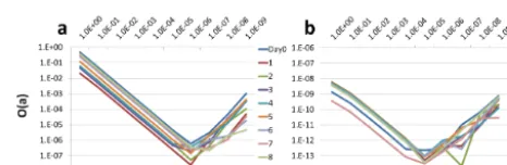
Figure 4 shows the results of the ratio of norms for the two major modules. The horizontal and vertical axes are re-spectively the values of the scaling factor a and the resid-ual O(a)for the ratio of norms in Eq. (2). The slopes with different colors show the residualO(a)calculated at differ-ent days. The numerical results show that, for all cases, the slopes are decreased as the scaling factor a is decreased, even if there are small differences of the magnitude tween the slopes. As expected, when the scaling factor be-comes smaller, the perturbation reaches the machine pre-cision and the slopes do not decrease anymore. With vari-ously different perturbations and initial conditions, the sim-ilar pattern described as in Fig. 4 shows the residual O(a)
for all other modules, including the main time-stepping loop module, prim_run_subcycle that is composed of the time-stepping module prim_advance_exp, along with two major modules shown in Fig. 4. This implies that the linearization for all nonlinear modules is performed properly and com-pletely. The TLM is verified to be accurate, and its solutions are therefore expected to be truly asymptotically correct. 3.2 Field checks
Further to verify the correctness of the TLM, we plotted the full field of V-wind components for the TLM and the
19 1
Figure 4. Linearity test for the two major modules: (a) compute_and_apply_rhs, and (b) 2
advance_hypervis. The horizontal and vertical axes are respectively the values of the scaling 3
factor a and the residual O(a) for the ratio of norms in Eq. (2). The slopes with different 4
colors show the residual O(a) calculated at different days. 5
6
Figure 4. Linearity test for the two major modules: (a) com-pute_and_apply_rhs, and (b) advance_hypervis. The horizontal and
vertical axes are respectively the values of the scaling factoraand the residualO(a)for the ratio of norms in Eq. (2). The slopes with different colors show the residualO(a)calculated at different days.
corresponding difference fields between the two nonlinear model forecasts. In general, an increment produced by as-similating any DA systems is believed to represent a typi-cal analysis error and is treated as a reasonable initial per-turbation, or the increment can be constructed by a differ-ence field between two full states in different forecast ranging (Ehrendorder and Errico, 1995). Because the magnitudes of the latter method are similar to those of the nonlinear model results at day 6 with reduced magnitude of 10 or 1 %, ini-tial perturbations are obtained by choosing nonlinear model results with 10 or 1 % reduced magnitude. The initial pertur-bations are used as the initial condition for the TLM, and the two parallel nonlinear models are also integrated over time: one with the perturbations added to the initial condition and the other without the initial perturbation.
1180 S. Kim et al.: Development of a tangent linear model (version 1.0)
20 1
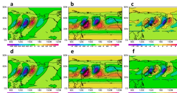
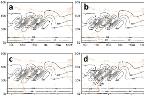
Figure 5. Evolution of different initial perturbations for the V-wind fields (m s-1). Upper panel 2
(a,b,c) shows wind with 10% perturbation of the initial state and lower panel (d,e,f) with 1% 3
perturbation (see details in Sect. 3.2). The shadings represent the difference between the two 4
nonlinear models runs with perturbed and unperturbed initial conditions. The contours 5
illustrate the evolution of wind perturbation propagated by the tangent linear model at 6
different times, the initial time (left column), 24h (middle), and 48h (right). 7
8
Figure 5. Evolution of different initial perturbations for the V-wind fields (m s−1). Upper panel (a, b, c) shows wind with 10 % perturbation of the initial state and lower panel (d, e, f) with 1 % perturbation (see details in Sect. 3.2). The shadings represent the difference between the two nonlinear models runs with perturbed and unperturbed initial conditions. The contours illustrate the evolution of wind perturbation propagated by the tangent linear model at different times, the initial time (left column), 24 h (middle), and 48 h (right).
2 also show linear trends between 10 and 1 % magnitudes of initial perturbations, and the pattern correlation with 1 % magnitude is much higher than that with 10 % magnitude. These results confirm that the initial evolution is well repre-sented by the developed TLM (version 1.0) up to at least 48 h for the resolution of 220 km (Ne=16). The similar numeri-cal results were obtained for different model configurations with different model resolutions, initial conditions, and per-turbations (figures are not shown). These results confirm that the TLM (version 1.0) for the HOMME dynamical core is correctly developed and reasonably well represents the ini-tial perturbation evolution.
3.3 Temporal increment
A time step size in tangent linear models plays an important role in numerical stability and computational cost, so it is important to choose a suitable time step size to balance be-tween the numerical stability and computational cost. A too short time step makes the TLM too expensive due to the I/O as seen in Sect. 2.4, and a too long time step makes the model numerically instable. There are a couple of ways to determine a proper time step size for stable integration of a TLM. One is to try different time step sizes for the TLM, and the other can check stability conditions for given numerical schemes.
Here, various time steps are applied to the TLM and empir-ically tested for numerical instabilities. Figure 6 shows snap-shots of V-wind fields at time 5 h for the results of the TLM with different time step sizes from1t=150 s to1t=600 increased by 150. At the time step of 1t=300, the result shows the stable time integration of the TLM up to 48 h, and the TLM with 1t=450 holds the numerical stability for 11 h. The TLM with time step of 1t=600 shows the
instability after 5 h. For a given 6 h assimilation window that is usually used for 4DVar schemes in many NWP centers, the TLM results with time step sizes less than1t=450 yield stable integration results and produce very similar results to those with default time stop of1t=450. Thus, the expanded time step size of1t=450 would be appropriate for a best temporal increment. This can be confirmed quantitatively by considering the relative mean error, defined, for any quantity
Xat the timeT =5 h, as
kXTLM−XNLDk/kXNLDk, (3)
whereXTLM is a TLM field atT =5 h,XNLD is the corre-sponding difference fields between the two nonlinear model forecasts at 5 h, andk kis a spatial averaged norm. Table 1 gives these values for the mean of the stat variable X at timeT =5 h. And the total wall-clock time is decreased, as the time step size is increased such that when1t=150 s is set to be 100 %, 21t becomes 56 %, 31t is 36 %, and 41t
for 33 %. Although the TLM (version 1.0) developed in this study still needs further improvement for its performance, the current version is practical within a scope of a reasonable compromise between linearity, computational efficiency, and forecast performances.
4 Summary and discussion
21 1
Figure 6. V-wind fields (ms-1) of the tangent linear model with different time increments at 5 2
hour later. Time step size ∆t is a) 150, b) 300, c) 450, d) 600 second. 3
4
5
Figure 6. V-wind fields (m s−1)of the tangent linear model with different time increments at 5 h later. Time step size1tis (a) 150,
(b) 300, (c) 450, and (d) 600 s.
trajectory of the nonlinear system, and also provides a com-putationally efficient way to calculate the model trajectory. Since the TLM is primarily intended to approximate the evo-lution of perturbations in a corresponding nonlinear model, the accuracy of the TLM is considered to be a measure of the model performance. In that regard, the developed codes for the TLM are checked by the Taylor–Lagrange formula and by comparison of time-evolved perturbation fields for the TLM with the difference fields between two controlled nonlinear model runs. Overall verification of the numerical results indicates that the tangent linear model is correctly de-veloped.
Generally, there are some major inaccuracy issues in de-veloping TLMs (Errico et al., 1993) due to the finite mag-nitude of the perturbations in initial/boundary conditions, model parameters, the strong nonlinearities, discontinuities in nonlinear models, and numerical instabilities, which make difficult the development of efficient and well-behaving tan-gent linear codes. During the development of the tantan-gent lin-ear codes for the HOMME dynamical core, however, we have not experienced any significant difficulty such as a tendency to suddenly grow small perturbations due to some unintended discontinuities or ill-conditioning in the HOMME model. We believe that it is because the dynamics has good computa-tional properties such as no singularity on both poles (Dennis et al., 2012).
Since the TLM requires nonlinear solutions as coefficients, the I/O strategy is important for the practical implication of the TLM. Two TLMs are developed with different I/O such as recalculating the basic state and storing the trajectories in file. The TLM with recalculating the basic state at ev-ery time step is extremely burdensome, but the results of the TLM well represent the evolution of perturbations, and those results can be used as reference fields in comparison with those of the approximated TLM. The extra burden leads to the alternate strategy for the TLM that is to store and read
Table 1. Relative mean errors.
Variable 1·1t 2·1t 3·1t 4·1t
u 0.0124556 0.0128355 0.0135081 0.163502
v 0.0128028 0.0120578 0.0115803 0.13647
t 0.00696689 0.00650514 0.00596657 0.104771
ps 0.00697304 0.00639369 0.00547336 0.0750567
the trajectories from the file. As the time step of the TLM is increased, the burden of I/O is decreased. Furthermore, given a time step size the instability during the TLM time integra-tion should be carefully studied. It is because the time step used of the developed TLM is directly used for the time step of the adjoint model, and it also influences the performance of 4DVar schemes.
The critical element in any operational prediction schemes such as 4DVar and four-dimensional ensemble-based varia-tional method (4DEnVar) will, of course, be the initializa-tion procedure. The issue that has not been addressed by the present development is the analysis increments in the ini-tialization procedure that generally develop gravity waves. To filter out high-frequency waves, an incremental analysis-updating scheme (Polavarapu et al., 2004) is developed for the forecast model, and for 4DEnVar and 4DVar. The TLM (version 1.0) developed here can be another option for an in-ternal digital filtering initialization scheme such that the high frequency in the analysis increments are filtered out by prop-agating the TLM forwards and backwards (with a negative time step), and then by forming a weighted average of the states in the combined trajectory. Korea Institute of Atmo-spheric Prediction Systems (KIAPS) is a government-funded nonprofit research and development institute currently devel-oping a four-dimensional ensemble-based variational method (4DEnVar). KIAPS will test the TLM (version 1.0) for the initialization procedure.
Code availability
All codes in the current version of TLM are available upon the request. Any potential user interested in those modules should contact B.-J. Jung, and any feedback on them is wel-come. Note that one may need help using the TLM model optimally, but we do not have the resources to support the model in an open way. Since ADM is currently being devel-oped based on the current version of TLM, all codes of ADM are also presumably available upon the request.
Acknowledgements. This work has been carried out through the
1182 S. Kim et al.: Development of a tangent linear model (version 1.0)
Also, we would like to thank the anonymous reviewers for their careful reading of the manuscript and their thoughtful comments that helped to clarify aspects of the manuscript.
Edited by: D. Ham
References
Bennett, A. F.: Inverse modeling of the ocean and atmosphere, Cam-bridge University Press, CamCam-bridge, 2002.
Courtier, P. and Talagrand, O.: Variational assimilation of meteoro-logical observations with the adjoint equation –Part I. Numerical results, Q. J. Roy. Meteorol. Soc., 113, 1329–1347, 1987. Courtier, P., Thepaut, J.-N., and Hollingworth, A.: A strategy for
operational implementation of 4D-Var, using an incremental ap-proach, Q. J. Roy. Meteorol. Soc., 120, 1367–1387, 1994. Dennis, J. M., Edwards, J., Evans, K. J., Guba, O. N., Lauritzen,
P. H., Mirin, A. A., St-Cyr, A., Taylor, M. A., and Worley, P. H.: CAM-SE: A scalable spectral element dynamical core for the Community Atmosphere Model, Int. J. High. Perform. C., 26, 74–89, 2012.
Ehrendorder, M. and Errico, R. M.: Mesoscale predictability and the spectrum of optimal perturbations, J. Atmos. Sci., 52, 3475– 3500, 1995.
Errico, R. and Raeder, K.: An examination of the accuracy of the linearization of a mesoscale model with moist physics, Q. J. Roy. Meteorol. Soc., 120, 1367–1387, 1999.
Errico, R. M., Vukicevic, T., and Raeder, K.: Examination of the accuracy of a tangent linear model, Tellus A, 45, 462–497, 1993. Giering, R. and Kaminski, T.: Recipes for adjoint code construction,
ACM T. Math. Software, 24, 437–474, 1998.
Jablonowski, C. and Williamson D. L.: A baroclinic wave test case for atmospheric model dynamical cores, Q. J. Roy. Meteorol. Soc., 132, 2943–2957, 2006.
Lacarra, J.-F. and Talagrand, O.: Short-range evolution of small per-turbations in a barotropic model, Tellus A, 40, 81–95, 1988. Nair, R. D. and Tufo, H. M.: Petascale atmospheric general
circulation models, J. Phys., 78, 012078, doi:10.1088/1742-6596/78/1/012078, 2007.
Nair, R. D., Choi, H.-W., and Tufo, H. M.: Computational aspects of a scalable high-order discontinuous Galerkin atmospheric dy-namical core, Comput. Fluids, 38, 309–319, 2009.
Navon, I. M., Zou, X., Derber, J., and Sela, J.: Variational data as-similation with an adiabatic version of the NMC spectral model, Mon. Weather Rev., 120, 1433–1446, 1992.
Polavarapu, S., Ren, S., Clayton, A. M., Sankey, D., and Rochon, Y.: On the relationship between incremental analysis updating and incremental digital filtering, Mon. Weather Rev., 132, 2495– 2502, 2004.
Rabier, F. and Courtier, P.: Four-Dimensional assimilation in the presence of baroclinic instability, Q. J. Roy. Meteorol. Soc., 118, 649–672, 1992.
Thomas, S. J. and Loft, R. D.: Semi-implicit spectral element model, J. Sci. Comput., 17, 339–350, 2002.
Yannick, T.: Diagnostics of linear and incremental approximations in 4D-Var, Q. J. Roy. Meteorol. Soc., 130, 2233–2251, 2004. Yannick T.: Incremental 4D-Var convergence study, Tellus, 59A,
706–718, 2007.
Zhu, J. and Kamachi, M.: The role of time step size in numeri-cal stability of tangent linear models, Mon. Weather Rev., 128, 1562–1572, 2000.