www.geosci-model-dev.net/10/1363/2017/ doi:10.5194/gmd-10-1363-2017
© Author(s) 2017. CC Attribution 3.0 License.
Global 7 km mesh nonhydrostatic Model Intercomparison Project
for improving TYphoon forecast (TYMIP-G7): experimental design
and preliminary results
Masuo Nakano1, Akiyoshi Wada2, Masahiro Sawada2, Hiromasa Yoshimura2, Ryo Onishi1, Shintaro Kawahara1, Wataru Sasaki1, Tomoe Nasuno1, Munehiko Yamaguchi2, Takeshi Iriguchi2, Masato Sugi2, and Yoshiaki Takeuchi2 1Japan Agency for Marine-Earth Science and Technology, 3173-25 Showa-machi, Kanazawa-ku,
Yokohama, Kanagawa 236-0001, Japan
2Meteorological Research Institute, Japan Meteorological Agency, 1-1 Nagamine, Tsukuba, Ibaraki 305-0052, Japan
Correspondence to:Masuo Nakano ([email protected])
Received: 11 July 2016 – Discussion started: 2 August 2016
Revised: 3 February 2017 – Accepted: 3 February 2017 – Published: 31 March 2017
Abstract. Recent advances in high-performance computers facilitate operational numerical weather prediction by global hydrostatic atmospheric models with horizontal resolutions of ∼10 km. Given further advances in such computers and the fact that the hydrostatic balance approximation becomes invalid for spatial scales<10 km, the development of global nonhydrostatic models with high accuracy is urgently re-quired.
The Global 7 km mesh nonhydrostatic Model Intercom-parison Project for improving TYphoon forecast (TYMIP-G7) is designed to understand and statistically quantify the advantages of high-resolution nonhydrostatic global atmo-spheric models to improve tropical cyclone (TC) predic-tion. A total of 137 sets of 5-day simulations using three next-generation nonhydrostatic global models with horizon-tal resolutions of 7 km and a conventional hydrostatic global model with a horizontal resolution of 20 km were run on the Earth Simulator. The three 7 km mesh nonhydrostatic mod-els are the nonhydrostatic global spectral atmospheric Dou-ble Fourier Series Model (DFSM), the Multi-Scale Simula-tor for the Geoenvironment (MSSG) and the Nonhydrostatic ICosahedral Atmospheric Model (NICAM). The 20 km mesh hydrostatic model is the operational Global Spectral Model (GSM) of the Japan Meteorological Agency.
Compared with the 20 km mesh GSM, the 7 km mesh models reduce systematic errors in the TC track, intensity and wind radii predictions. The benefits of the multi-model ensemble method were confirmed for the 7 km mesh
nonhy-drostatic global models. While the three 7 km mesh models reproduce the typical axisymmetric mean inner-core struc-ture, including the primary and secondary circulations, the simulated TC structures and their intensities in each case are very different for each model. In addition, the simulated track is not consistently better than that of the 20 km mesh GSM. These results suggest that the development of more sophis-ticated initialization techniques and model physics is needed to further improve the TC prediction.
1 Introduction 1.1 Global model
Forecasts (ECMWF) has operated a global model with a horizontal resolution of 9 km since March 2016. Therefore, sooner or later, it is expected that all numerical weather pre-diction centres will operate global models with horizontal grid intervals of<10 km.
Developing high-resolution models with a horizontal grid spacing of<10 km must resolve three challenges. The first is to use a nonhydrostatic equation system. In the Earth’s atmosphere, hydrostatic balance is established for spatial scales>10 km with high accuracy. Therefore, the primitive equation system, which approximates the vertical momen-tum equation with the hydrostatic balance equation, has been used in conventional global models. The second challenge is to use a dynamical core that effectively runs on state-of-the-art, massively parallel computer systems. Many conventional global models use the spectral method in which the Legen-dre transform is used for the meridional expansion of cer-tain prognostic variables. Because the computational cost of this transform increases with the third power of the number of grid points and communication costs become large, one solution is to avoid such transforms (Tomita et al., 2001). The last challenge is to implement sophisticated physical schemes suitable for high-resolution models, especially for clouds, because they can be partially resolved in a model with a horizontal resolution of 10 km.
Because developing operational numerical weather pre-diction models with high accuracy requires huge computa-tional and human resources, the concept of transition of re-search to operations (R2O) has recently been encouraged. For example, the Hurricane Weather Research and Forecast-ing Model (Bernardet et al., 2015) and an atmosphere–ocean coupled limited-area model (Ito et al., 2015) have been devel-oped based on R2O in the United States and Japan, respec-tively. In Japan, two next-generation, nonhydrostatic global atmospheric models have already been developed and used in the research community. These are called the Multi-Scale Simulator for the Geoenvironment (MSSG) and the Nonhy-drostatic ICosahedral Atmospheric Model (NICAM). In ad-dition, the Meteorological Research Institute (MRI) of the Japan Meteorological Agency (JMA) has developed a next-generation nonhydrostatic atmospheric model called the non-hydrostatic global spectral atmospheric Double Fourier Se-ries Model (DFSM). To gain knowledge, to develop and im-prove nonhydrostatic global models and to share them with the research and operational communities are some aims of the present project.
1.2 TC forecasts
Tropical cyclones (TCs) are characterized by violent winds and torrential rain. These events cause tremendous dam-age to human lives, property and socioeconomic activity via landslides, floods and storm surges. Because an average of 26 TCs (>30 % of the global average) form in the western North Pacific each year, accurate TC track and intensity
fore-casts are of great concern to east Asian countries to mitigate the impacts of the associated disasters. The JMA has the pri-mary responsibility for TC forecasts in the western North Pa-cific region as a Regional Specialized Meteorological Cen-tre (RSMC) of the World Meteorological Organization. The JMA has operated a 20 km mesh global atmospheric model to predict weather and TC tracks and intensities since 2007. Therefore, upgrading their global atmospheric model is a promising approach to improve TC forecasts in the western North Pacific.
Errors in TC track prediction by the JMA operational global atmospheric model at a given lead time have decreased on an average by half over the past 20 years (JMA, 2014) as the operational model has been upgraded. For example, TC track prediction error in a 30 h forecast with a 60 km mesh global model was∼200 km in 1997 and decreased to
∼100 km in 2010 with a 20 km mesh model. Even though we have continuously improved TC track prediction, abnormally large track prediction errors called “forecast busts” (e.g. Carr and Elsberry, 2000) still occur. Typhoons Conson (2004) (Ya-maguchi et al., 2009) and Fengshen (2008) (Yamada et al., 2016; Nasuno et al., 2016) are typical examples. Tracks pre-dicted by tens-of-kilometres mesh global models for Feng-shen predicted recurvature far from the Philippines; however, the typhoon made landfall in the Philippines according to best-track analyses (Joint Typhoon Warning Center, 2008). Yamada et al. (2016) reported that a 3.5 km mesh next-generation nonhydrostatic global model successfully simu-lated its landfall in the Philippines. Increases in the horizon-tal resolution of global atmospheric models with appropriate physical schemes can potentially reduce bust cases and an-nual mean errors of TC track predictions.
1.3 TYMIP-G7
The primary objectives of the Global 7 km mesh nonhy-drostatic Model Intercomparison Project for improving TY-phoon forecast (TYMIP-G7) are to understand and statisti-cally quantify the advantages of high-resolution global atmo-spheric models towards the improvement of TC track and in-tensity forecasts. The project is conducted as a strategic pro-gram of the Earth Simulator of the Japan Agency for Marine-Earth Science and Technology (JAMSTEC). We accomplish this objective via a model intercomparison of three 7 km mesh nonhydrostatic atmospheric models (DFSM, MSSG and NICAM) and a 20 km mesh hydrostatic operational at-mospheric model of the JMA (Global Spectral Model; GSM) in various cases. Because a huge amount of data is produced by each model, we developed an effective method to handle and visualize the data. Sharing the knowledge obtained in this project with research and operational communities will facilitate R2O.
In this paper, we describe the specifications of TYMIP-G7 and the set of metrics used to validate the model perfor-mances. Some preliminary results concerning the metrics are also shown. This paper comprises six sections. Section 2 de-scribes the common experimental design, including the cases and the output dataset. Section 3 briefly overviews the scien-tific outcomes of each model and describes the detailed spec-ifications. Section 4 presents the metrics, analysis method and visualization. Preliminary results concerning the advan-tages of high-resolution models for TC prediction and the simulated TC wind structure are given in Sect. 5. Section 6 is devoted to conclusions and future work.
2 Experimental design
We imitated JMA operational specifications to conduct 5-day numerical experiments with the models (DFSM, GSM, MSSG and NICAM). The JMA 6-hourly global objective analysis data were used for each model to derive atmospheric initial conditions. The data were provided based on the GSM grid system, a linear Gaussian grid with a horizontal reso-lution of 20 km and a hybrid sigma-pressure vertical coordi-nate. DFSM and GSM interpolated data directly onto their model grids, whereas MSSG and NICAM preliminarily in-terpolated the data onto common latitude–longitude grids and pressure levels and then interpolated this to their model grids. A merged satellite and in situ data global daily sea sur-face temperature (SST) product with a horizontal resolution of 0.25◦(Kurihara et al., 2006) was used for the SST oceanic initial conditions and the sea ice concentration. Because an atmospheric model was used in the present study, SSTs for the 5-day integration were given as the boundary conditions. It was assumed that an SST anomaly from an observed daily climatology on an initial date persisted during the 5-day pe-riod. Even though no diurnal cycle of SST was input into the
models, NICAM can simulate the diurnal cycle because it is coupled with a simple bulk ocean model, as described later.
The project was implemented using the Earth Simulator, a supercomputer system operated by JAMSTEC. The Earth Simulator is based on NEC SX-ACE, a distributed-memory, massively parallel vector system with a total of 5120 com-putational nodes. Each node has one central processing unit, which comprises four processing cores and a 64 GB main memory. The theoretical peak performance of the entire sys-tem is 1.3 peta floating-point operations per second.
2.1 Cases
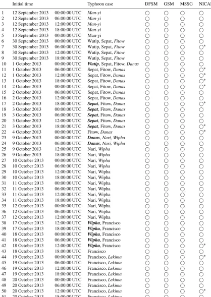
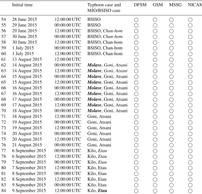
We conducted the project for two stages: from June 2015 to September 2015 and from October 2015 to March 2016. The first stage addressed TCs from September to October in 2013, during the most active TC season since 1951. We fore-casted nine TCs in 52 runs (Table 1). However, we detected some flaws in MSSG and NICAM, and we could not per-form some of the numerical experiments. The second stage addressed the life cycle of a TC, e.g. genesis, rapid inten-sification, recurvature and extratropical transition in addi-tion to the Madden–Julian oscillaaddi-tion (MJO; Madden and Ju-lian, 1972) and the boreal summer intraseasonal oscillation (BSISO; Wang and Rui, 1990; Wang and Xie, 1997). After we improved the detected flaws, we examined 13 TCs in 85 runs (Table 2) in addition to the numerical experiments in the first stage. We analyse the model output obtained in the second stage in this paper.
2.2 Dataset
Table 1.List of initial times for stage 1 of TYMIP-G7. Typhoon cases in italic font are weaker than a tropical storm and those in bold italic font are extratropical cyclones.
Initial time Typhoon case DFSM GSM MSSG NICAM
1 12 September 2013 00:00:00 UTC Man-yi 2 12 September 2013 06:00:00 UTC Man-yi 3 12 September 2013 12:00:00 UTC Man-yi 4 12 September 2013 18:00:00 UTC Man-yi 5 13 September 2013 00:00:00 UTC Man-yi 6 30 September 2013 00:00:00 UTC Wutip, Sepat,Fitow 7 30 September 2013 06:00:00 UTC Wutip, Sepat,Fitow ∗ 8 30 September 2013 12:00:00 UTC Wutip, Sepat,Fitow 9 30 September 2013 18:00:00 UTC Wutip, Sepat,Fitow 10 1 October 2013 00:00:00 UTC Wutip, Sepat, Fitow,Danas 11 1 October 2013 06:00:00 UTC Sepat, Fitow,Danas ∗ 12 1 October 2013 12:00:00 UTC Sepat, Fitow,Danas ∗ 13 1 October 2013 18:00:00 UTC Sepat, Fitow,Danas ∗ 14 2 October 2013 00:00:00 UTC Sepat, Fitow,Danas ∗ 15 2 October 2013 06:00:00 UTC Sepat, Fitow,Danas 16 2 October 2013 12:00:00 UTC Sepat, Fitow,Danas 17 2 October 2013 18:00:00 UTC Sepat, Fitow,Danas ∗ 18 3 October 2013 00:00:00 UTC Sepat, Fitow,Danas 19 3 October 2013 06:00:00 UTC Sepat, Fitow,Danas 20 3 October 2013 12:00:00 UTC Sepat, Fitow,Danas 21 3 October 2013 18:00:00 UTC Sepat, Fitow,Danas ∗ 22 4 October 2013 00:00:00 UTC Fitow,Danas ∗ 23 9 October 2013 00:00:00 UTC Danas,Nari, Wipha 24 9 October 2013 06:00:00 UTC Danas,Nari, Wipha 25 9 October 2013 12:00:00 UTC Nari,Wipha 26 9 October 2013 18:00:00 UTC Nari,Wipha 27 10 October 2013 00:00:00 UTC Nari,Wipha 28 10 October 2013 06:00:00 UTC Nari,Wipha 29 10 October 2013 12:00:00 UTC Nari, Wipha 30 10 October 2013 18:00:00 UTC Nari, Wipha 31 11 October 2013 00:00:00 UTC Nari, Wipha 32 11 October 2013 06:00:00 UTC Nari, Wipha 33 11 October 2013 12:00:00 UTC Nari, Wipha 34 11 October 2013 18:00:00 UTC Nari, Wipha 35 12 October 2013 00:00:00 UTC Nari, Wipha 36 12 October 2013 06:00:00 UTC Nari, Wipha 37 12 October 2013 12:00:00 UTC Nari, Wipha 38 17 October 2013 12:00:00 UTC Wipha, Francisco 39 17 October 2013 18:00:00 UTC Wipha, Francisco 40 18 October 2013 00:00:00 UTC Wipha, Francisco 41 18 October 2013 06:00:00 UTC Wipha, Francisco 42 18 October 2013 12:00:00 UTC Wipha, Francisco ∗ 43 18 October 2013 18:00:00 UTC Francisco 44 19 October 2013 00:00:00 UTC Francisco,Lekima ∗ 45 19 October 2013 06:00:00 UTC Francisco,Lekima 46 19 October 2013 12:00:00 UTC Francisco,Lekima 47 19 October 2013 18:00:00 UTC Francisco,Lekima 48 20 October 2013 00:00:00 UTC Francisco,Lekima 49 20 October 2013 06:00:00 UTC Francisco,Lekima 50 20 October 2013 12:00:00 UTC Francisco,Lekima ∗ 51 20 October 2013 18:00:00 UTC Francisco,Lekima 52 21 October 2013 00:00:00 UTC Francisco,Lekima
Table 2.List of initial times for stage 2 of TYMIP-G7. Typhoon cases in italic font are weaker than a tropical storm and those in bold italic font are extratropical cyclones.
Initial time Typhoon case and DFSM GSM MSSG NICAM∗ MJO/BSISO case
Table 2.Continued.
Initial time Typhoon case and DFSM GSM MSSG NICAM∗ MJO/BSISO case
54 28 June 2015 12:00:00 UTC BSISO 55 29 June 2015 00:00:00 UTC BSISO 56 29 June 2015 12:00:00 UTC BSISO,Chan-hom 57 30 June 2015 00:00:00 UTC BSISO,Chan-hom 58 30 June 2015 12:00:00 UTC BSISO, Chan-hom 59 1 July 2015 00:00:00 UTC BSISO, Chan-hom 60 1 July 2015 12:00:00 UTC BSISO, Chan-hom 61 13 August 2015 12:00:00 UTC 62 14 August 2015 00:00:00 UTC Molave,Goni,Atsani 63 14 August 2015 12:00:00 UTC Molave,Goni,Atsani 64 15 August 2015 00:00:00 UTC Molave, Goni, Atsani 65 15 August 2015 12:00:00 UTC Molave, Goni, Atsani 66 16 August 2015 00:00:00 UTC Molave, Goni, Atsani 67 16 August 2015 12:00:00 UTC Molave, Goni, Atsani 68 17 August 2015 00:00:00 UTC Molave, Goni, Atsani 69 17 August 2015 12:00:00 UTC Molave, Goni, Atsani 70 18 August 2015 00:00:00 UTC Molave, Goni, Atsani 71 18 August 2015 12:00:00 UTC Goni, Atsani 72 19 August 2015 00:00:00 UTC Goni, Atsani 73 19 August 2015 12:00:00 UTC Goni, Atsani 74 20 August 2015 00:00:00 UTC Goni, Atsani 75 20 August 2015 12:00:00 UTC Goni, Atsani 76 21 August 2015 00:00:00 UTC Goni, Atsani 77 6 September 2015 00:00:00 UTC Kilo,Etau 78 6 September 2015 12:00:00 UTC Kilo,Etau 79 7 September 2015 00:00:00 UTC Kilo,Etau 80 7 September 2015 12:00:00 UTC Kilo, Etau 81 8 September 2015 00:00:00 UTC Kilo, Etau 82 8 September 2015 12:00:00 UTC Kilo, Etau 83 9 September 2015 00:00:00 UTC Kilo, Etau 84 9 September 2015 12:00:00 UTC Kilo,Etau 85 10 September 2015 00:00:00 UTC Kilo,Etau
∗Run with the fixed version of MATSIRO (Sect. 2.2.3).
3 Models
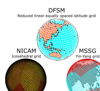
We used three 7 km mesh nonhydrostatic global atmospheric models in TYMIP-G7 (Fig. 1). The DFSM was developed in the MRI of the JMA. The MSSG was developed at JAM-STEC. NICAM was developed at JAMSTEC, the University of Tokyo and the RIKEN Advanced Institute for Computa-tional Science. In addition, we used GSM with a horizontal grid spacing of ∼20 km to quantify the advantages of the higher-resolution models. DFSM and GSM are spectral mod-els and MSSG and NICAM are grid modmod-els. The following subsections detail the aforementioned models (Table 4) and the experimental design.
3.1 GSM and DFSM
GSM (JMA, 2013) is a hydrostatic global spectral atmo-spheric model using atmo-spherical harmonics. The JMA has used
this model operationally to provide fundamental informa-tion for forecasts. The model was put into operainforma-tion in 1988 with T63L16 resolution (200 km mesh), where “Tx” refers to the horizontal triangular spectral truncation with a total wavenumber x using a quadratic Gaussian grid and “Ly” refers to the number of vertical layersy. The resolution of the operational GSM increased to T106L21 (120 km mesh) in 1989, T213L30 (60 km mesh) in 1996, T213L40 in 2001, TL319L40 (60 km mesh) in 2005, TL959L60 (20 km mesh) in 2007 and TL959L100 in 2014 (JMA, 2016), where “TLx” refers to the horizontal triangular spectral truncation with a total wavenumberx using a linear Gaussian grid (Hortal, 2002).
Table 3.Output variables and domains.
Domain Interval Variable Horizontal
resolution
Global 1 h accumulated cloud ice (cldi), accumulated cloud water (cldw), outward longwave radiation (olr), sea level pressure (psea), 2 m specific humid-ity (qs), sea surface temperature (sst), total precipitable water (tpw), 2 m temperature (ts), 10 m zonal wind speed (us), 10 m meridional wind speed (vs)
1.25◦
1 h (average) latent heat flux (fllh), zonal wind stress (flmu), meridional wind stress (flmv), sensible heat flux (flsh), precipitation (prc), precipitation by cumulus parameterization (prcc)
1.25◦
3 h cloud cover (cvr), cloud water content (cwc), cloud water (qc or xc), cloud ice (qi or xi), rain water (qr or xr), snow (qs or xs), graupel (qg or xg), specific humidity (q), relative humidity (rh), temperature (t), zonal wind speed (u), meridional wind speed (v), vertical wind speed (w), height (z)
1.25◦
3 h (average) cumulus-induced heating (hrcv), cloud-induced heating (hrlc), radiation-induced heating (hrr), turbulence-induced heating (hrvd), cumulus-induced moistening (qrcv), cloud-induced moistening (qrlc), radiation-induced heating (qrvd), cumulus-induced zonal acceleration (urcv), turbulence-induced zonal acceleration (urvd), cumulus-induced meridional acceleration (vrcv), turbulence-induced meridional acceler-ation (vrvd)
1.25◦
Western North 1 h cldi, cldw, olr, psea, qs, sst, tpw, ts, us, vs ∼7 km
Pacific/tropics 1 h (average) fllh, flmu, flmv, flsh, prc, prcc ∼7 km
3 h cvr, cwc,q, rh,t,u,v,w,z ∼7 km
3 h (average) hrcv, hrlc, hrr, hrvd, qrcv, qrlc, qrvd, urcv, urvd, vrcv, vrvd ∼7 km
for the research community. TIGGE data have been used for various applications, including TC track prediction (Yam-aguchi et al., 2012, 2015) and the MJO (Matsueda and Endo, 2011). In addition, GSM has been used to produce atmo-spheric reanalysis datasets, i.e. the Japanese 25-year ReAnal-ysis (JRA-25; Onogi et al., 2007) and the Japanese 55-year ReAnalysis (JRA-55; Kobayashi et al., 2015). MRI global climate models have been developed based on GSM and have been used in climate research, such as global warming pro-jections (e.g. Mizuta et al., 2006; Yukimoto et al., 2011) and stratospheric studies (e.g. Shibata et al., 1999). TC activity in future climates has been intensively studied using vari-ous model physics and horizontal resolutions (Murakami and Sugi, 2010; Murakami et al., 2012a, b).
The MRI developed DFSM by changing the hydrostatic dynamical core of GSM using spherical harmonics to a nonhydrostatic dynamical core using a double Fourier se-ries (Yoshimura, 2012). DFSM uses the same basis func-tions of the double Fourier series as Cheong (2000). In DFSM, a fast Fourier transform is used instead of a Legen-dre transform in the meridional direction. Because the com-putational cost of the fast Fourier transform is much smaller than that of the Legendre transform, especially at high
res-DFSM
Reduced linear equally spaced latitude grid
NICAM
Icosahedral grid Yin-Yang grid
MSSG
Figure 1.Schematic diagram of the horizontal grid structures of the three models used in TYMIP-G7.
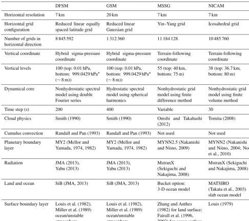
Table 4.Brief description of the specifications for each global nonhydrostatic model.
DFSM GSM MSSG NICAM
Horizontal resolution 7 km 20 km 7 km 7 km
Horizontal grid configuration
Reduced linear equally spaced latitude grid
Reduced linear Gaussian grid
Yin–Yang grid Icosahedral grid
Number of grids in horizontal direction
8 845 592 1 312 360 11 184 128 10 485 760
Vertical coordinate Hybrid sigma-pressure coordinate
Hybrid sigma-pressure coordinate
Terrain-following coordinate
Terrain-following coordinate
Vertical levels 100 (top: 0.01 hPa, bottom: 999.0429 hPa∗ (∼8 m))
100 (top: 0.01 hPa, bottom: 999.0429 hPa∗ (∼8 m))
55 (top: 40 km, bottom: 75 m)
38 (top: 36.7 km, bottom: 80 m)
Dynamical core Nonhydrostatic spectral model using double Fourier series
Hydrostatic spectral model using spherical harmonics
Nonhydrostatic grid model using finite difference method
Nonhydrostatic grid model using finite volume method
Time step (s) 200 400 Variable 30
Cloud physics Smith (1990) Smith (1990) Onishi and Takahashi (2012)
Tomita (2008)
Cumulus convection Randall and Pan (1993) Randall and Pan (1993) Not used Not used
Planetary boundary layer
MY2 (Mellor and Yamada, 1974, 1982)
MY2 (Mellor and Yamada, 1974, 1982)
MYNN2.5 (Nakanishi and Niino, 2009)
MYNN2 (Nakanishi and Niino, 2004; Noda et al., 2010)
Radiation JMA (2013), Yabu (2013)
JMA (2013), Yabu (2013)
MstranX (Sekiguchi and Nakajima, 2008)
MstranX (Sekiguchi and Nakajima, 2008)
Land and ocean SiB (JMA, 2013) SiB (JMA, 2013) Bucket option: 3-D ocean model
MATSIRO (Takata et al., 2003) slab ocean model
Surface boundary layer Louis et al. (1982), Miller et al. (1989) ocean/unstable atmosphere
Louis et al. (1982), Miller et al. (1989) ocean/unstable atmosphere
Zhang and Anthes (1982) for land surface; Fairall et al. (1996, 2003) for ocean surface
Louis (1979)
∗Full-level pressure for surface pressure=1000 hPa.
60 km resolution model was shown by Yoshimura and Mat-sumura (2005).
In GSM and DFSM, a two-time-level, implicit, semi-Lagrangian scheme (e.g. Hortal, 2002) is used to facilitate long time steps for computational efficiency. The vertically conservative semi-Lagrangian scheme is used in the advec-tion calculaadvec-tion (Yoshimura and Matsumura, 2003, 2005; Yukimoto et al., 2011), and a correction method similar to that described by Priestley (1993) and Gravel and Stani-forth (1994) is used for global conservation in the material transport. To save computational costs, we used a reduced grid (Miyamoto, 2006) in which the number of zonal grid points is decreased, especially at high latitudes (Fig. 1).
scheme (Yoshimura, 2012). Recalculation is necessary only for the non-constant linear terms during the iteration. It is found that only a single iteration is sufficient for conver-gence.
Physical packages included in GSM and DFSM are the same as those in the March 2014 version of the opera-tional global atmospheric model of the JMA. A prognostic cumulus parameterization scheme (Randall and Pan, 1993) and other schemes in GSM are used in DFSM without any changes. The physical process is described in detail in the JMA (2013).
3.2 MSSG
MSSG is an atmosphere–ocean coupled nonhydrostatic model aimed at a seamless simulation from global to local scales (Takahashi et al., 2006, 2013). The MSSG comprises atmospheric (MSSG-A) and oceanic (MSSG-O) compo-nents. MSSG uses a conventional lat–long grid system for re-gional simulations and the Yin–Yang grid system (Kageyama and Sato, 2004; Baba et al., 2010), which comprises two overlapping lat–long grids to avoid the polar singularity problem, for global simulations. MSSG has been used in a wide range of applications. A cloud-system-resolving global ocean–atmosphere coupled MSSG successfully simulated an observed MJO propagation (Sasaki et al., 2016). A global atmosphere–ocean coupled experiment with 11 km horizon-tal resolution with a nested region with 2.7 km horizonhorizon-tal res-olution simulated sea surface cooling caused by a TC along its track (Takahashi et al., 2013). High-resolution regional atmospheric simulations have been conducted to investigate the influence of the choice of cloud microphysics scheme and in-cloud turbulence on cloud development (Onishi et al., 2011, 2012). MSSG-O with a 2 km horizontal resolu-tion has been used to investigate the dispersion of radionu-clides released from the Fukushima Daiichi nuclear power plant (Choi et al., 2013) and the effect of wind on long-term summer water temperature trends in Tokyo Bay, Japan, with 200 m horizontal resolution (Lu et al., 2015). MSSG-A with a 5 m spatial resolution has been used in building-resolving urban atmosphere simulations to examine the heat environ-ments of streets (Takahashi et al., 2013).
In this study, MSSG-A is exclusively used. Its dynam-ical core is based on the nonhydrostatic equations, and it predicts the three wind components, as well as air density and pressure. Each horizontal computational domain cov-ers 4056×1352 grids in the Yin–Yang lat–long grid sys-tem. The average horizontal grid spacing is 7 km. The ver-tical level comprises 55 verver-tical layers with a top height of 40 km and the lowermost vertical layer at 75 m. The third-order Runge–Kutta scheme is used for time integration. The fast terms related to acoustic and gravity waves are calculated separately with a shorter time step (Wicker and Skamarock, 2002). A fifth-order upwind scheme (Wicker and Skamarock, 2002) was chosen for the momentum advection and a
second-order weighted average flux scheme with the Superbee flux limiter (Toro, 1989) for the scalar advection. For turbulent diffusion, the Mellor–Yamada–Nakanishi–Niino level 2.5 scheme (Nakanishi and Niino, 2009) was used. The MSSG-Bulk model (Onishi and Takahashi, 2012), a six-category bulk cloud microphysics model, is used for explicit cloud physics. Model simulation radiation transfer code version 10 (MstranX; Sekiguchi and Nakajima, 2008) is used to calcu-late longwave and shortwave radiation transfer.
During the first stage of the project, extraordinary in-creases in precipitable water appeared in the 5-day inte-grations when the conventional bulk surface flux model of Zhang and Anthes (1982) was used for both land and ocean surfaces. This issue was solved by the use of the COARE 3.0 model (Fairall et al., 1996, 2003) for ocean surface fluxes with Zhang and Anthes (1982) being used only for land sur-face fluxes. This combination was used for all simulations in the second stage, and we plan to rerun all the simulations in the first stage.
3.3 NICAM
NICAM (Satoh et al., 2008, 2014) was developed as a cli-mate model and can explicitly resolve clouds without any convective parameterization, which is known to be the most ambiguous component in conventional climate models (Ran-dall et al., 2003). From the first appearance of realistic cloud-resolving simulations using a 3.5 km mesh horizontal reso-lution by Miura et al. (2007a), NICAM has primarily been used to study tropical meteorological systems, such as the MJO (Miura et al., 2007b; Nasuno, 2013; Miyakawa et al., 2014), TC genesis from the MJO in boreal winter (Fudeyasu et al., 2008, 2010a, b), TC genesis from the BSISO in the western North Pacific (Oouchi et al., 2009; Nakano et al., 2015) and BSISO in the northern Indian Ocean (Taniguchi et al., 2010; Yanase et al., 2010). NICAM has also been used for quasi-real-time forecast systems during field ob-servation campaigns to support field obob-servations (Nasuno, 2013). Recent progress with high-performance computing infrastructures, such as the K-computer, a 10-petaflop super-computer in Japan, facilitates 870 m mesh global simulations (Miyamoto et al., 2013, 2015; Kajikawa et al., 2016). This is the highest resolution to date (10 July 2016). Climate simula-tions (of 30 years) using a 14 km mesh model (Kodama et al., 2015) and large member (10 240 members) ensemble data as-similations based on an ensemble Kalman filter (Miyoshi et al., 2015) have also been executed.
horizon-tal resolution of g-level 10, corresponding to a 7 km mesh. The vertical level comprises 38 vertical layers to a top height of 36.7 km with the lowest layer at 80 m. NICAM uses a fully compressible nonhydrostatic equation system for the dynamics of the atmosphere. The model uses an icosahedral grid system in the horizontal direction with the Arakawa A-grid and terrain-following coordinate with the Lorenz A-grid in the vertical direction. The equations are discretized us-ing the flux form of the finite volume method. The numer-ical scheme guarantees conservation of total mass and en-ergy. The second-order Runge–Kutta scheme is primarily used for time integration, whereas the third-order Runge– Kutta scheme is used in some cases to avoid computational instability. NICAM uses the split-explicit scheme together with the horizontal explicit and vertical implicit scheme to avoid the restriction of the Courant–Friedrichs–Lewy condi-tion for acoustic waves. The NICAM Single-moment Wa-ter 6 cloud microphysics scheme (Tomita, 2008) is used for cloud microphysics without any convective parameter-ization. Planetary boundary layer processes are calculated using the Mellor–Yamada–Nakanishi–Niino level 2 scheme (Nakanishi and Niino, 2004) implemented and examined by Noda et al. (2010). Longwave and shortwave radiation trans-fer is calculated using MstranX (Sekiguchi and Nakajima, 2008). Land surface processes are computed by the Mini-mal Advanced Treatments of Surface Interaction and Runoff (MATSIRO; Takata et al., 2003). NICAM is coupled with a simple slab ocean model. This model calculates SST based on the local heat balance between the ocean slab and the atmosphere, and the other ocean dynamics, such as verti-cal mixing and advection, are not considered. The slab has a specific heat capacity determined by its thickness (15 m). The calculated SST is nudged with a persistent SST anomaly with an e-folding time of 7 days. The surface flux is calcu-lated by the Louis (1979) scheme with sea surface roughness length parameterization by Moon et al. (2007).
During the first stage of this project, there were frequent problems of divisions by zero in MATSIRO that had not been experienced in simulations with coarser horizontal resolu-tions. This issue was fixed before simulations in the second stage, and abnormal cases in the first stage had to be rerun. The fix had a slight impact on the prediction results. During the second stage, however, two cases were still unable to be completed due to numerical instability (Table 2).
4 Metrics, analysis methods and visualization 4.1 Metrics
Here, we define the following metrics to evaluate the TC forecast performance:
1. computational resources for a 5-day forecast on the Earth Simulator (node hours),
2. TC track (position) error every 6 h of forecast time (km), 3. TC intensity (central pressure) error every 6 h of
fore-cast time (hPa),
4. averaged radius of surface 50-knot (25 m s−1) wind (AR50) error (km), and
5. averaged radius of surface 30-knot (15 m s−1) wind (AR30) error (km).
It is important for the operational model that the calcu-lation is completed in less time with smaller computational resources so that we applied metric (1). The metrics (2)–(5) measure the accuracy of the track, intensity and surface wind structure prediction based on the RSMC Tokyo best-track data.
4.2 TC tracking
We extract TC tracks from the model experiments using the hourly mean sea level pressure (SLP) data with a horizon-tal resolution of∼7 km for DFSM, MSSG and NICAM and 20 km for GSM. A TC centre is defined as a minimum SLP point from the predicted mean SLP field smoothed 100 times by a 1–2–1 filter for each longitude and latitude. The ini-tial TC centre is defined within a radius of 1◦from a centre position based on the RSMC Tokyo best-track data. The next centre position is defined as the minimum SLP point from the smoothed SLP field within a radius of 1◦from the previous centre position. The tracking terminates when the minimum SLP points reach a proximity of 1◦from the lateral boundary in the domain of the output data or the difference between the minimum SLP and an ambient SLP defined as an areal average within 500 km of the minimum SLP point is less than 1 hPa. The tracking algorithm works well for nearly all cases; however, misdetection occurred for some very weak TCs. These cases were excluded from the validation. 4.3 AR50 and AR30
The RSMC Tokyo best-track data contain longest and short-est radii of 50-knot and 30-knot wind speeds and their di-rection. AR50 and AR30 are defined as the average of the longest and shortest radii of the 50-knot and 30-knot wind speeds, respectively. The directions of the longest and short-est radii are defined by eight directions (N, NE, E, SE, S, SW, W and NW) in the best-track data. Therefore, we calculated the radii of the 50-knot and 30-knot wind in the model in each of the eight directions first and then determined the direction of the longest and shortest radii. Then, the radii in those two directions were averaged to obtain AR50 and AR30. 4.4 Multi-model ensemble mean
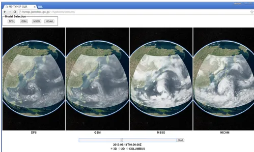
Figure 2.Screen capture of the web application: outgoing longwave radiation at 14 September 2013, 10:00:00 UTC, simulated in experiments initialized at 12 September 2013, 06:00:00 UTC.
MME is a simple ensemble average derived from a combi-nation of individual models, which reduces the average fore-cast error relative to the best individual predictions by the in-dividual models. MME also provides additional information about the forecast uncertainty, enhancing forecast confidence (Goerss, 2000; Yamaguchi et al., 2012).
4.5 Visualization
We developed a web application that allows the simulta-neous visualization of multi-model results. Figure 2 shows a screen capture of this application, which portrays digi-tal globes using Cesium.js (Analytical Graphics, Inc., http: //cesiumjs.org), a WebGL-based virtual globe and map en-gine. Visualization results of each model are overlaid on them. We used the Volume Data Visualizer for Google Earth (VDVGE; Kawahara, 2012; Kawahara et al., 2015) to de-pict visualization results for the overlay. VDVGE is origi-nally a visualization software that exports visualization re-sults in the KML format, a data format suitable for Google Earth. An option to export in the CZML format, suitable for Cesium.js, has recently been implemented in VDVGE. The present web application enables us to view the animation display for time-series visualization results of each model while synchronously changing the three-dimensional view-point. An option to display each model result selectively is
also available. This application enables the four models to be easily compared.
5 Results
5.1 Computational resources
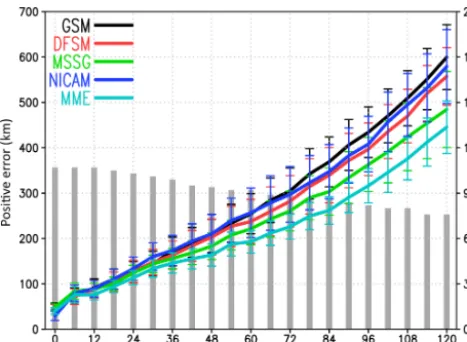
Figure 3.Errors in the track prediction for GSM, DFSM, MSSG, NICAM and MME (in the second stage). Each grey bar indicates the number of samples at each forecast time (right-vertical axis). Error bars indicate 95 % confidence levels of the central pressure difference between the prediction and the RSMC Tokyo best-track data.
5.2 Track predictions
To quantify the advantage of using finer resolutions for TC track prediction, we examined the time series of TC track prediction errors with reference to the RSMC Tokyo best track for the second stage (Fig. 3). TC track predictions by DFSM, MSSG and NICAM performed better than GSM. However, the reduction in the track errors depended on the TC case. That is, the use of finer resolution alone does not always improve TC track prediction. This suggests that im-provements in the initial conditions and those of the physical processes in each model are also required to improve track prediction.
We also validated MME using track predictions of the three models with reference to the RSMC Tokyo best-track data. MME track prediction gave the smallest track errors for forecast time (FT) of 24–120 h. The reduction rate of the MME position error from that of GSM was ∼26% at FT=120 h relative to that of GSM. The position error of MME at that FT corresponds to that of GSM at FT=96 h. Even though MME had promising results with regard to improving TC track prediction, future work is required to achieve more robust results and to answer scientific and prac-tical questions, such as in which cases MME is effective and why.
5.3 Intensity predictions
Figure 4 shows time series of the average central pressure and the standard deviation in each model relative to the RSMC Tokyo best-track data for the second stage. Because the global objective analysis data, which were used as initial con-ditions of the numerical experiments, tend to reproduce TC
Figure 4.Errors in the predictions of the central pressure for GSM, DFSM, MSSG, NICAM and MME (in the second stage). Each grey bar indicates the number of samples at each forecast time (right-vertical axis). Error bars indicate 95 % confidence levels of the central pressure difference between the prediction and the RSMC Tokyo best-track data.
central pressure shallower than those in RSMC Tokyo best-track data, cases with an initial bias<20 hPa are validated. The central pressures in MSSG and NICAM showed rela-tively small biases compared to the error in GSM. These re-sults indicate that these 7 km mesh models help decrease sys-tematic positive errors for the central pressure. However, the central pressure in DFSM showed over-intensification and the magnitude of the bias after FT=54 h became larger than that in GSM. Because both DFSM and GSM had the same specifications except for the horizontal resolution, this result suggests that the improvement of physics schemes suitable for such high-resolution models is needed for accurate fore-casts of the central pressure. GSM showed a gradual growth of positive bias in the central pressure until FT=84 h, in-cluding the initial 24 h, when the 7 km mesh models showed a continuous reduction in the errors. After this early reduc-tion, the errors of the 7 km mesh models began to grow in model-specific ways. MSSG showed a gradual growth of positive bias in the central pressure until FT=84 h and then the errors become saturated. NICAM retained nearly no bias for the central pressure until FT=84 h and then showed a slight growth in the negative bias for the central pressure until FT=120 h. DFSM had a gradual growth of negative bias for the central pressure until FT=120 h. MME showed a nega-tive bias for the central pressure after FT=24 h.
5.4 Predictions of the TC wind structure
Figure 5.Errors in the averaged radius of the 50-knot wind (AR50) for GSM, DFSM, MSSG, NICAM and MME (in the second stage). Each grey bar indicates the number of samples at each forecast time (right-vertical axis). Error bars indicate 95 % confidence levels of the AR50 difference between the prediction and the RSMC Tokyo best-track data.
at the initial time. This negative bias is partially attributed to the shallower estimation of the central pressure by ∼5 hPa (Fig. 4) associated with the biases in the global objective analysis data, which were used as initial conditions of the numerical experiments. The difference in the interpolation methods to prepare the initial data for each model might also affect the bias. The negative biases of all 7 km mod-els decrease in the early stage. The negative bias of DFSM monotonically decreases until FT=78 h and then saturates at∼25 km at FT=78–120 h. The bias of MSSG decreases more rapidly until FT=48 h and becomes positive until FT=84 h and then returns to a negative bias of∼20 km. The bias of NICAM continuously decreases until FT=66 h and then becomes positive. At FT=120 h, NICAM shows a positive bias of 40 km, which was a smaller magnitude than that of the initial bias. Conversely, GSM shows little improvement in the negative bias so that its negative bias remains at∼60 km at FT=120 h. These results show that high-resolution models can significantly reduce the error of AR50. In addition, MME has a promising result in improv-ing the AR50 prediction: MME showed a bias of nearly zero for FT=60–120 h.
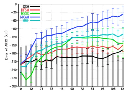
Figure 6 shows the validation results of AR30. All models show a negative bias of more than 200 km at FT=0 h. The negative biases of all 7 km models tended to decrease in the early stage as FT proceeded. The negative bias of DFSM de-creases to 180 km by FT=36 h and then relatively slowly de-creases to 150 km by FT=120 h. The negative bias of MSSG temporarily increases in the first 6 h, and then decreases. The bias of NICAM continuously decreases up to FT=120 h, re-sulting in a negative bias as small as 35 km at FT=120 h. GSM had little improvement in AR30 up to FT=96 h and
Figure 6.Errors in the averaged radius of the 30-knot wind (AR30) for GSM, DFSM, MSSG, NICAM and MME (in the second stage). Each grey bar indicates the number of samples at each forecast time (right-vertical axis). Error bars indicate 95 % confidence levels of the AR30 difference between the prediction and the RSMC Tokyo best-track data.
shows a negative bias of∼170 km at FT=120 h. These re-sults show that high-resolution models can also reduce the error in AR30. However, all the models still had relatively large negative biases compared to the error in AR50. Towards a better prediction of TC wind structure, further improve-ments in the quality of the objective analysis and the models themselves are needed. The bias of MME also decreases up to FT=120 h; however, its magnitude is larger than that of NICAM. Interestingly, DFSM tended to simulate the small wind radii (AR50 and AR30) despite the largest negative bias for central pressure. NICAM and MSSG, which had smaller biases for central pressure, tended to simulate larger wind radii than DFSM. Therefore, it is expected that simu-lated TCs in NICAM and MSSG have horizontally broader structure than that in DFSM. These results imply that internal dynamics of modelled TC are significantly different among those models. Further studies are needed to understand the differences in internal dynamics of modelled TC by chang-ing physics parameterization and dynamical core.
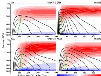
Figure 7.Composite analysis of the radius-height cross section of the axisymmetric mean radial (shaded) and tangential (contour) wind speed for TCs at the time of the analysed central pressure between 920 and 940 hPa in the RSMC Tokyo best-track data. Contour intervals are 5 m s−1(values greater than 15 m s−1are plotted). The green line depicts the RMW between 850 and 200 hPa. The grey shading at the bottom of each panel is below the surface.
for all models. While all 7 km mesh models reproduced typ-ical axisymmetric mean inner-core structures, such as pri-mary and secondary circulations, the simulated TC structures differed significantly between the 7 km models as expected above. The TCs calculated by DFSM had the highest maxi-mum tangential wind speed and the smallest radius of max-imum wind (RMW) of the models. In addition, its primary circulation was the deepest, reaching up to 100 hPa in the ver-tical direction and the narrowest in the horizontal direction. The depth of the inflow and outflow layers in DFSM was rel-atively thin and had the strongest radial velocity. The TCs in NICAM and MSSG showed relatively similar structures to each other; however, MSSG had thicker inflow and outflow layers. Differences in the heating and inertial stability in the inner core led to differences in the primary and secondary circulation (Shapiro and Willoughby 1982). Understanding the cause of the differences in the simulated structures in the models will lead to improvements in all the models.
6 Conclusions and future work
TYMIP-G7 was implemented in two stages from June 2015 through March 2016. The aim of the project was to sta-tistically quantify and understand the advantages of high-resolution global atmospheric models to improve 5-day TC track, intensity and wind radii forecasts. We performed
nu-merical experiments for multiple TC cases in 137 runs using three 7 km mesh global nonhydrostatic atmospheric models: DFSM, MSSG and NICAM. We also included a 20 km mesh global hydrostatic atmospheric model, GSM, on the Earth Simulator of JAMSTEC. We statistically evaluated errors in the TC track, intensity and wind radii predictions with the following primary results.
(C1) The 7 km models statistically improve both the TC in-tensity and track predictions, whereas the improvement in the individual TC tracks depends on the case. (C2) The MME is a promising approach to further enhance
the TC track and AR50 predictions.
(C3) The predicted TC structure differs greatly between the three models even though they have the same horizontal resolution.
To follow up the above results to further improve TC pre-diction, we must answer the following questions.
(Q1) Why are the TC predictions improved by high-resolution models?
To answer (Q1), an intercomparison of forecasts by the 20 km mesh GSM and the 7 km mesh models (DFSM, MSSG and NICAM) is the first step. Concerning (Q2), the predicted TC structure depends on the physics schemes, such as cloud microphysics, planetary boundary layer and surface flux, as well as the dynamical core of the model. To understand the impacts of the model physics schemes, sensitivity experi-ments altering the schemes and/or tuning parameters will be required.
In addition, the following topics are suggested for future work:
(F1) extended-range forecasts, contributing to TC genesis and MJO/BSISO forecasts;
(F2) atmosphere–ocean coupled experiments to examine im-pacts on TC intensity and track and MJO/BSISO; (F3) further high-resolution experiments to study impacts of
better inner-core representation on TC intensities and tracks; and
(F4) data assimilation to contribute for validating the models and understanding the TC processes and model initial-izations.
These topics are addressed below.
An advantage of global models for TC prediction over limited-area models is the coverage of multi-scale atmo-spheric phenomena from a mesoscale vortex to synoptic en-vironments. Because TC genesis strongly depends on syn-optic environments modulated by the MJO/BSISO, global models should be used for its forecasting. Indeed, Nakano et al. (2015) and Xiang et al. (2015) showed that TC gene-sis is predictable up to 2 weeks in advance; this great skill in TC genesis forecasting was attributed to its strong ability to forecast BSISO/MJO. We are conducting extended-range (longer than 2 weeks) forecast experiments using the four models in several cases and will investigate the advantage of high-resolution modes.
In the present project, atmosphere-only models were used, except for NICAM, which is coupled with a simple slab ocean model. However, studies have shown that fully cou-pled atmosphere–ocean processes are essential for especially slow-moving, intense TCs (e.g. Yablonsky and Ginis, 2009). Recently, Zarzycki (2016) reproduced sea surface cooling caused by TCs realistically using a global atmospheric model coupled with a slab ocean model with a simple parameteri-zation of ocean turbulent mixing, which is not considered in NICAM, and demonstrated that the cooling led to signif-icant reduction in TC intensity. These processes affect the TC structure and therefore the track and intensity. In addi-tion, a fully coupled atmosphere–ocean model is better for MJO/BSISO forecasts. MSSG is already capable of cou-pling MSSG-A with MSSG-O (Sasaki et al., 2016; Taka-hashi et al., 2013). In addition, NICAM has been coupled
with the Center for Climate System Research Ocean COm-ponent Model (COCO; Hasumi, 2006). Therefore, we will use these coupled global models to examine the impacts of global atmosphere–ocean processes on TC forecasts.
To improve the high-resolution models, the validation of simulated phenomena using observations is essential. An understanding of the essential processes and the modelling therefore requires high-resolution spatiotemporal observa-tions. Recent advances in satellite observations furnish quan-titatively and qualitatively rich observational data. However, the spatiotemporal resolution is still insufficient for the vali-dation of TC structures simulated by high-resolution models. Aggressively developing data assimilation techniques using satellite observations (e.g. Zhang et al., 2016; Okamoto et al., 2016) is a promising means of obtaining high-resolution, spatiotemporal, three-dimensional TC structures, including those at the cloud convection scale (∼O (1 km)). In addition, applying such cloud-resolving analyses to deriving the initial conditions of high-resolution models may improve TC pre-diction.
7 Data availability
Access to the initial and boundary data for the models and model outputs can be granted upon request, under a collab-orative framework between MRI, JAMSTEC and related in-stitutes or universities.
Competing interests. The authors declare that they have no conflict of interest.
Acknowledgements. This project was conducted as “The Earth Simulator Strategic Project with Special Support” of JAMSTEC. All numerical experiments were run on the Earth Simulator (NEC SX-ACE). This study was partly supported by HPCI Strategic Programs for Innovative Research (SPIRE) Field 3, the FLAGSHIP 2020 project of the Ministry of Education, Culture, Sports, Science and Technology (MEXT) and KAKENHI 26282111, 26400475 and 15K05292 of the Japan Society for the Promotion of Science (JSPS). The authors thank Mikiko Ikeda, Yuichi Saitoh and Hiromitsu Fuchigami for supporting the experiments on the Earth Simulator. The authors also acknowledge Hideaki Kawai and Eiki Shindo for the fruitful discussions. The schematic diagram of the NICAM grid was provided by Masaki Satoh.
Edited by: P. Ullrich
References
Baba, Y., Takahashi, K., Sugimura, T., and Goto, K.: Dy-namical core of an atmospheric general circulation model on a yin–yang grid, Mon. Weather Rev., 138, 3988–4005, doi:10.1175/2010MWR3375.1, 2010.
Bénard, P., Vivoda, J., Mašek, J., Smolíková, P., Yessad, K., Smith, Ch., Brožková, R., and Geleyn, J.-F.: Dynamical kernel of the Aladin-NH spectral limited-area model: Revised formulation and sensitivity experiments, Q. J. Roy. Meteor. Soc., 136, 155–169, doi:10.1002/qj.522, 2010.
Bernardet, L., Tallapragada, V., Bao, S., Trahan, S., Kwon, Y., Liu, Q., Tong, M., Biswas, M., Brown, T., Stark, D., Carson, L., Yablonsky, R., Uhlhorn, E., Gopalakrishnan, S., Zhang, X., Mar-chok, T., Kuo, B., and Gall, R.: Community support and transi-tion of research to operatransi-tions for the hurricane weather research and Forecasting model, B. Am. Meteorol. Soc., 96, 953–960, doi:10.1175/BAMS-D-13-00093.1, 2015.
Braun, S. A. and Tao, W.-K.: Sensitivity of high-resolution simu-lations of Hurricane Bob (1991) to planetary boundary layer pa-rameterizations, Mon. Weather Rev., 128, 3941–3961, 2000. Bubnová, R., Hello, G., Bénard, P., and Geleyn, J.-F.: Integration of
the fully elastic equations cast in the hydrostatic pressure terrain-following coordinate in the framework of the ARPEGE/Aladin NWP system, Mon. Weather Rev., 123, 515–535, 1995. Carr III, L. E. and Elsberry, R. L.: Dynamical tropical
cy-clone track forecast errors, Part I: Tropical region error sources, Weather Forecast., 15, 641–661, doi:10.1175/1520-0434(2000)015<0641:DTCTFE>2.0.CO;2, 2000.
Cheong, H.-B.: Application of double Fourier series to the shallow-water equations on a sphere, J. Comput. Phys., 165, 261–287, 2000.
Choi, Y., Kida, S., and Takahashi, K.: The impact of oceanic cir-culation and phase transfer on the dispersion of radionuclides released from the Fukushima Dai-ichi Nuclear Power Plant, Biogeosciences, 10, 4911–4925, doi:10.5194/bg-10-4911-2013, 2013.
Fairall, C. W., Bradley, E. F., Rogers, D. P., Edson, J. B., and Young, G. S.: Bulk parameterization of air-sea fluxes for Tropical Ocean-Global Atmosphere Coupled-Ocean Atmosphere Response Ex-periment, J. Geophys. Res., 101, 747–764, 1996.
Fairall, C. W., Bradley, E. F., Hare, J. E., Grachev, A. A., and Ed-son, J. B.: Bulk parameterization of air-sea fluxes: updates and verification for the COARE algorithm, J. Climate, 16, 571–591, 2003.
Fierro, A. O., Rogers, R. F., Marks, F. D., and Nolan, D. S.: The impact of horizontal grid spacing on the microphysical and kinematic structures of strong tropical cyclones simulated with the WRF-ARW model, Mon. Weather Rev., 137, 3717–3743, doi:10.1175/2009MWR2946.1, 2009.
Fudeyasu, H., Wang, Y., Satoh, M., Nasuno, T., Miura, H., and Yanase, W.: Global cloud-system-resolving model NICAM suc-cessfully simulated the lifecycles of two real tropical cyclones, Geophys. Res. Lett., 35, L22808, doi:10.1029/2008GL036003, 2008.
Fudeyasu, H., Wang, Y., Satoh, M., Nasuno, T., Miura, H., and Yanase, W.: Multiscale interactions in the life cycle of a tropi-cal cyclone simulated in a global cloud-system-resolving model, Part I: Large-scale and storm-scale evolutions, Mon. Weather Rev., 138, 4285–4304, doi:10.1175/2010MWR3474.1, 2010a.
Fudeyasu, H., Wang, Y., Satoh, M., Nasuno, T., Miura, H., and Yanase, W.: Multiscale interactions in the life cycle of a tropi-cal cyclone simulated in a global cloud-system-resolving model, Part II: System-scale and mesoscale processes, Mon. Weather Rev., 138, 4305–4327, doi:10.1175/2010MWR3475.1, 2010b. Gentry, M. S. and Lackmann, G. M.: Sensitivity of simulated
tropi-cal cyclone structure and intensity to horizontal resolution, Mon. Weather Rev., 138, 688–704, doi:10.1175/2009MWR2976.1, 2010.
Goerss, J. S.: Tropical cyclone track forecasts using an ensemble of dynamical models, Mon. Weather Rev., 128, 1187–1193, doi:10.1175/1520-0493(2000)128<1187:TCTFUA>2.0.CO;2, 2000.
Gravel, S. and Staniforth, A.: A mass-conserving semi-Lagraingian scheme for the shallow-water equations, Mon. Weather Rev., 122, 243–248, 1994.
Hasumi, H.: CCSR Ocean Component model (COCO) version 4.0. CCSR Rep 25, The University of Tokyo, Chiba, Japan, 2006. Hortal, M.: The development and testing of a new
two-time-level semi-Lagrangian scheme (SETTLS) in the ECMWF forecast model, Q. J. Roy. Meteor. Soc., 128, 1671–1687, doi:10.1002/qj.200212858314, 2002.
Ito, K., Kuroda, T., Saito, K., and Wada, A.: Forecasting a large number of tropical cyclone intensities around Japan using a high-resolution atmosphere–ocean coupled model, Weather Forecast., 30, 793–808, doi:10.1175/WAF-D-14-00034.1, 2015.
Japan Meteorological Agency (JMA): Outline of the operational nu-merical weather prediction at the Japan Meteorological Agency, Appendix to WMO technical progress report on the global data-processing and forecasting system and numerical weather pre-diction, 188 pp., available at: http://www.jma.go.jp/jma/jma-eng/ jma-center/nwp/outline2013-nwp/index.htm, 2013.
Japan Meteorological Agency: Annual report on the activities of the RSMC Tokyo-typhoon center, 90 pp., available at: http://www.jma.go.jp/jma/jma-eng/jma-center/rsmc-hp-pub-eg/ AnnualReport/2014/Text/Text2014.pdf, 2014.
Japan Meteorological Agency: The upgrade history of the global spectral model, available at: http://www.wis-jma.go.jp/ddb/ latest_modelupgrade.txt, 2016.
Joint Typhoon Warning Center: 2008 Annual tropical cyclone re-port, 116 pp., available at: http://www.usno.navy.mil/NOOC/ nmfc-ph/RSS/jtwc/atcr/2008atcr.pdf, 2008.
Kageyama, A. and Sato, T.: The Yin-Yang grid: An overset grid in spherical geometry, Geochem. Geophys. Geosyst., 5, Q09005, doi:10.1029/2004GC000734, 2004.
Kajikawa, Y., Miyamoto, Y., Yoshida, R., Yamaura, T., Yashiro, H., and Tomita, H.: Resolution dependence of deep convections in a global simulation from over 10-kilometer to sub-kilometer grid spacing, Prog. Earth Planet. Sci., 3, 16, doi:10.1186/s40645-016-0094-5, 2016.
Kanada, S. and Wada, A.: Numerical study on the extremely rapid intensification of an intense tropical cyclone, Typhoon Ida (1958), J. Atmos. Sci., 72, 4194–4217, doi:10.2151/jmsj.2015-037, 2015.
Kawahara, S., Onishi, R., Goto, K., and Takahashi, K.: Realistic representation of clouds in Google Earth, Proc. SIGGRAPH Asia 2015 VHPC, doi:10.1145/2818517.2818541, 2015.
Kobayashi, S., Ota, Y., Harada, Y., Ebita, A., Moriya, M., Onoda, H., Onogi, K, Kamahori, H., Kobayashi, C., Endo, H., Miyaoka, K., and Takahashi, K.: The JRA-55 reanalysis: General specifi-cations and basic characteristics, J. Meteor. Soc. Jpn., 93, 5–48, doi:10.2151/jmsj.2015-001, 2015.
Kodama, C., Yamada, Y., Noda, A. T., Kikuchi, K., Kajikawa, Y., Nasuno, T., Tomita, T., Yamaura, T., Takahashi, T. G., Hara, M., Kawatani, Y., Satoh, M., and Sugi, M.: A 20-year climatology of a NICAM AMIP-type simulation, J. Meteor. Soc. Jpn., 93, 393– 424, doi:10.2151/jmsj.2015-024, 2015.
Kurihara, Y., Sakurai, T., and Kuragano, T.: Global daily sea sur-face temperature analysis using data from satellite microwave radiometer, satellite infrared radiometer and in-situ observations, Weather Bull., 73, s1–s18, 2006 (in Japanese).
Louis, J. F.: A parametric model of vertical eddy fluxes in the atmo-sphere, Bound.-Lay. Meteor., 2, 187–202, 1979.
Louis, J. F., Tiedtke, M., and Geleyn, J. F.: A short history of the operational PBL parameterization at ECMWF, Proc. Workshop on Planetary Boundary Layer Parameterization, Reading, UK, ECMWF, 59–79, 1982.
Lu, L.-F., Onishi, R., and Takahashi, K.: The effect of wind on long-term summer water temperature trends in Tokyo Bay, Japan, Ocean Dynam., 65, 919–930, doi:10.1007/s10236-015-0848-4, 2015.
Madden, R. A. and Julian, P. R.: Description of global-scale circu-lation cells in the tropics with a 40–50 day period, J. Atmos. Sci., 29, 1109–1123, 1972.
Matsueda, M. and Endo, H.: Verification of medium-range MJO forecasts with TIGGE, Geophys. Res. Lett., 38, L11801, doi:10.1029/2011GL047480, 2011.
Mellor, G. L. and Yamada, T.: A hierarchy of turbulence closure models for planetary boundary layers, J. Atmos. Sci., 31, 1791– 1806, 1974.
Mellor, G. L. and Yamada, T.: Development of a turbulence clo-sure model for geophysical fluid problems, Rev. Geophys. Space Phys., 20, 851–875, 1982.
Miller, M. J., Palmer, T. N., and Swinbank, R.: Parameterization and influence of subgridscale orography in general circulation and numerical weather prediction models, Meteor. Atmos. Phys., 40, 84–109, 1989.
Miura, H., Satoh, M., Tomita H., Noda, A. T., Nasuno, T., and Iga, S.: A short-duration global cloud-resolving simulation with a re-alistic land and sea distribution, Geophys. Res. Lett., 34, L02804, doi:10.1029/2006GL027448, 2007a.
Miura, H., Satoh, M., Nasuno T., Noda, A. T., and Oouchi, K.: A Madden-Julian oscillation event realistically simulated by a global cloud-resolving model, Science, 318, 1763–1765, doi:10.1126/science.1148443, 2007b.
Miyakawa, T., Satoh, M., Miura, H., Tomita, H., Yashiro, H., Noda, A. T., Yamada, Y., Kodama, C., Kimoto, M., and Yoneyama, K.: Madden-Julian oscillation prediction skill of a new-generation global model demonstrated using a supercomputer, Nat. Comm., 5, 3769, doi:10.1038/ncomms4769, 2014.
Miyamoto, K.: Introduction of the reduced Gaussian grid into the operational global NWP model at JMA, CAS/JSC WGNE
Re-search Activities in Atmospheric and Ocean Modelling, 36, 6.9– 6.10, 2006.
Miyamoto, Y., Kajikawa, Y., Yoshida, R., Yamaura, T., Yashiro, H., and Tomita, H.: Deep moist atmospheric convection in a subkilo-meter global simulation, Geophys. Res. Lett., 40, 4922–4926, doi:10.1002/grl.50944, 2013.
Miyamoto, Y., Yoshida, R., Yamaura, T., Yashiro, H., Tomita, H., and Kajikawa, Y.: Does convection vary in different cloud distur-bances?, Atmos. Sci. Lett., 16, 305–309, doi:10.1002/asl2.558, 2015.
Miyoshi, T., Kondo, K., and Terasaki, K.: Big ensemble data assim-ilation in numerical weather prediction, Computer, 48, 15–21, doi:10.1109/MC.2015.332, 2015.
Mizuta, R., Oouchi, K., Yoshimura, H., Noda, A., Katayama, K., Yukimoto, S., Hosaka, M., Kusunoki, S., Kawai, H., and Nak-agawa, M.: 20-km-mesh global climate simulations using JMA-GSM model – mean climate states, J. Meteor. Soc. Jpn., 84, 165– 185, doi:10.2151/jmsj.84.165, 2006.
Moon, I.-J., Ginis, I., Hara, T., and Thomas, B.: A physics-based parameterization of air–sea momentum flux at high wind speeds and its impact on hurricane intensity predictions, Mon. Weather Rev., 135, 2869–2878, doi:10.1175/MWR3432.1, 2007. Murakami, H. and Sugi, M.: Effect of model resolution
on tropical cyclone climate projections, SOLA, 6, 73–76, doi:10.2151/sola.2010-019, 2010.
Murakami, H., Mizuta, R., and Shindo, E.: Future changes in tropical cyclone activity projected by physics and multi-SST ensemble experiments using the 60-km-mesh MRI-AGCM, Clim. Dynam., 39, 2569–2584, doi:10.1007/s00382-011-1223-x, 2012a.
Murakami, H., Wang, Y., Yoshimura, H., Mizuta, R., Sugi, M., Shindo, E., Adachi, Y., Yukimoto, S., Hosaka, M., Kusunoki, S., Ose, T., and Kitoh, A.: Future changes in tropical cyclone activ-ity projected by the new high-resolution MRI-AGCM, J. Climate, 25, 3237–3260, doi:10.1175/JCLI-D-11-00415.1, 2012b. Nakanishi, M. and Niino, H.: An improved Mellor-Yamada
level-3 model with condensation physics: Its design and verification, Bound.-Lay. Meteor., 112, 1–31, 2004.
Nakanishi, M. and Niino, H.: Development of an Improved Tur-bulence Closure Model for the Atmospheric Boundary Layer, J. Meteor. Soc. Jpn., 87, 895–912, doi:10.2151/jmsj.87.895, 2009. Nakano, M., Nasuno, T., Sawada, M., and Satoh, M.: Intraseasonal
variability and tropical cyclogenesis in the western North Pa-cific simulated by a global nonhydrostatic atmospheric model, Geophys. Res. Lett., 42, 565–571, doi:10.1002/2014GL062479, 2015.
Nasuno, T.: Forecast skill of Madden–Julian oscillation events in a global nonhydrostatic model during the CINDY2011/DYNAMO observation period, SOLA, 9, 69–73, doi:10.2151/sola.2013-016, 2013.
Nasuno, T., Yamada, H., Nakano, M., Kubota, H., Sawada, M., and Yoshida, R.: Global cloud-permitting simulations of Typhoon Fengshen (2008), Geosci. Lett., 3, 32, doi:10.1186/s40562-016-0064-1, 2016.
Okamoto, K., Aonashi, K., Kubota, T., and Tashima, T.: Experimen-tal assimilation of the GPM-Core DPR reflectivity profiles for Typhoon Halong (2014), Mon. Weather Rev., 144, 2307–2326, doi:10.1175/MWR-D-15-0399.1, 2016.
Onishi, R. and Takahashi, K.: A warm-bin–cold-bulk hybrid cloud microphysical model, J. Atmos. Sci., 69, 1474–1497, doi:10.1175/JAS-D-11-0166.1, 2012.
Onishi, R., Takahashi, K., and Komori, S.: High-resolution simu-lations for turbulent clouds developing over the ocean, in: Gas Transfer at Water Surfaces, edited by: Komori, S., McGillis, W., and Kurose, R., Kyoto University Press, 6, 582–592, 2011. Onogi, K., Tsutsui, J., Koide, H., Sakamoto, M., Kobayashi, S.,
Hat-sushika, H., Matsumoto, T., Yamazaki, N., Kamahori, H., Taka-hashi, K., Kadokura, S., Wada, K., Kato, K., Oyama, R., Ose, T., Mannoji, N., and Taira, R.: The JRA-25 Reanalysis, J. Meteor. Soc. Jpn., 85, 369-432, doi:10.2151/jmsj.85.369, 2007. Oouchi, K., Noda, A. T., Satoh, M., Miura, H., Tomita, H.,
Na-suno, T., and Iga, S.: A simulated preconditioning of typhoon genesis controlled by a boreal summer Madden-Julian Oscilla-tion event in a global cloud-resolving mode, SOLA, 5, 65–68, doi:10.2151/sola.2009-017, 2009.
Priestley, A.: A quasi-conservative version of the semi-Lagrangian advection scheme, Mon. Weather Rev., 121, 621–629, 1993. Randall, D. and Pan, D.-M.: Implementation of the
Arakawa-Schubert cumulus parameterization with a prognostic closure, The representation of cumulus convection in numerical models, AMS Meteor. Monogr. Series, 46, 137–144, 1993.
Randall, D., Khairoutdinov, M., Arakawa, A., and Grabowski, W.: Breaking the cloud parameterization deadlock, B. Am. Meteorol. Soc., 84, 1547–1564, doi:10.1175/BAMS-84-11-1547, 2003. Rogers, R. F., Reasor, P., and Lorsolo, S.: Airborne doppler
obser-vations of the inner-core structural differences between intensify-ing and steady-state tropical cyclones, Mon. Weather Rev., 141, 2970–2991, doi:10.1175/MWR-D-12-00357.1, 2013.
Sasaki, W., Onishi, R., Fuchigami, H., Goto, K., Nishikawa, S., Ishikawa, Y., and Takahashi, K.: MJO simulation in a cloud-system-resolving global ocean-atmosphere coupled model, Geo-phys. Res. Lett., 43, 9352–9360, doi:10.1002/2016GL070550, 2016.
Satoh, M., Matsuno, T., Tomita, H., Miura, H., Nasuno, T., and Iga, S.: Nonhydrostatic icosahedral atmospheric model (NICAM) for global cloud resolving simulations, J. Comput. Phys., 227, 3486– 3514, doi:10.1016/j.jcp.2007.02.006, 2008.
Satoh, M., Tomita, H., Yashiro, H., Miura, H, Kodama, C., Seiki, T., Noda, A. T., Yamada, Y., Goto, D., Sawada, M., Miyoshi, T., Niwa, Y., Hara, M., Ohno, T., Iga, S., Arakawa, T., Inoue, T., and Kubokawa, H.: The non-hydrostatic icosahedral atmospheric model: description and development, Prog. Earth Planet. Sci., 1, 18, doi:10.1186/s40645-014-0018-1, 2014.
Sekiguchi, M. and Nakajima, T.: A k-distribution-based radiation code and its computational optimization for an atmospheric gen-eral circulation model, J. Quant. Spectrosc. Ra., 109, 2779–2793, doi:10.1016/j.jqsrt.2008.07.013, 2008.
Shibata, K., Yoshimura, H., Ohizumi, M., Hosaka, M., and Sugi, M.: A simulation of troposphere, stratosphere and mesosphere with MRI/JMA98 GCM, Pap. Meteor. Geophys., 50, 15–53, 1999.
Shapiro, L. J. and Willoughby, H. E.: The response of balanced hur-ricanes to local sources of heat and momentum, J. Atmos. Sci., 39, 378–394, 1982.
Smith, R. N. B.: A scheme for predicting layer clouds and their water content in a general circulation model, Q. J. Roy. Meteor. Soc., 116, 435–460, 1990.
Takahashi, K., Peng, X., Ohnishi, R., Sugimura, T., Ohdaira, M., Goto, K., and Fuchigami, H.: Multi-scale weather/climate sim-ulations with Multi-Scale Simulator for the Geoenvironment (MSSG) on the Earth Simulator, Ann. Rep. Earth Simulator Cen-ter, April 2006–March 2007, 27–33, ISSN 1348–5822, 2006. Takahashi, K., Onishi, R., Baba, Y., Kida, S., Matsuda, K., Goto,
K., and Fuchigami, H.: Challenge toward the prediction of ty-phoon behaviour and down pour, J. Phys. Conference Series, 454, 012072, 2013.
Takata, K., Emori, S., and Watanabe, T.: Development of the minimal advanced treatments of surface interaction and runoff, Global Planet. Change, 38, 209–222, 2003.
Taniguchi, H., Yanase, W., and Satoh, M.: Ensemble simula-tion of cyclone Nargis by a global cloud-system-resolving model—modulation of cyclogenesis by the Madden-Julian oscil-lation, J. Meteor. Soc. Jpn., 88, 571–591, doi:10.2151/jmsj.2010-317, 2010.
Tomita, H.: New microphysical schemes with five and six categories by diagnostic generation of cloud ice, J. Meteorol. Soc. Jpn., 86, 121–142, doi:10.2151/jmsj.86A.121, 2008.
Tomita, H., Tsugawa, M., Satoh, M., and Goto, K.: Shal-low water model on a modified icosahedral geodesic grid by using spring dynamics, J. Comp. Phys., 174, 579–613, doi:10.1006/jcph.2001.6897, 2001.
Toro, E. F.: A weighted average flux method for hyperbolic conser-vation laws, P. R. Soc. London, 423, 401–418, 1989.
Wang, B. and Rui, H.: Synoptic climatology of transient tropical in-traseasonal convection anomalies: 1975–1985, Meteorol. Atmos. Phys., 44, 43–61, 1990.
Wang, B. and Xie, X.: A model for the boreal summer intraseasonal oscillation, J. Atmos. Sci., 54, 72–86, 1997.
Wang, H. and Wang, Y.: A numerical study of typhoon Megi (2010): Part I: Rapid intensification, Mon. Weather Rev., 142, 29–48, doi:10.1175/MWR-D-13-00070.1, 2014.
Wedi, N. P. and Smolarkiewicz, P. K.: A framework for testing global non-hydrostatic models, Q. J. Roy. Meteor. Soc., 135, 469–484, doi:10.1002/qj.377, 2009.
Wicker, L. J. and Skamarock, W. C.: Time-split-ting methods for elastic models using forward time schemes, Mon. Weather Rev., 130, 2088–2097, 2002.
Xiang, B., Lin, S.-J., Zhao, M., Zhang, S., Vecchi, G., Li, T., Jiang, X., Harris, L., and Chen, J.-H.: Beyond weather time-scale prediction for hurricane Sandy and super typhoon Haiyan in a global climate model, Mon. Weather Rev., 143, 524–535, doi:10.1175/MWR-D-14-00227.1, 2015.
Yablonsky, R. M. and Ginis, I.: Limitation of one-dimensional ocean models for coupled hurricane–ocean model forecasts, Mon. Weather Rev., 137, 4410–4419, doi:10.1175/2009MWR2863.1, 2009.
Yamada, H., Nasuno, T., Yanase, W., and Satoh, M.: Role of the vertical structure of a simulated tropical cyclone in its motion: A case study of Typhoon Fengshen (2008), SOLA, 12, 203–208, doi:10.2151/sola.2016-041, 2016.
Yamaguchi, M., Iriguchi, T., Nakazawa, T., and Wu, C.-C.: An ob-serving system experiment for Typhoon Conson (2004) using a singular vector method and DOTSTAR data, Mon. Weather Rev., 137, 2801–2816, 2009.
Yamaguchi, M., Nakazawa, T., and Hoshino, S.: On the relative ben-efits of a multi-centre grand ensemble for tropical cyclone track prediction in the western North Pacific, Q. J. Roy. Meteor. Soc., 138, 2019–2029, doi:10.1002/qj.1937, 2012.
Yamaguchi, M., Vitart, F., Lang, S. T. K., Magnusson, L., Elsberry, R. L., Elliott, G., Kyouda, M., and Nakazawa, T.: Global distribu-tion on the skill of tropical cyclone activity forecasts from short-to medium-range time scales, Weather Forecast., 30, 1695–1709, doi:10.1175/WAF-D-14-00136.1, 2015.
Yanase, W., Taniguchi, H., and Satoh, M.: The genesis of trop-ical cyclone Nargis (2008): Environmental modulation and numerical predictability, J. Meteor. Soc. Jpn., 88, 497–519, doi:10.2151/jmsj.2010-314, 2010.
Yoshimura, H.: Development of a nonhydrostatic global spectral at-mospheric model using double Fourier series, CAS/JSC WGNE Research Activities in Atmospheric and Ocean Modeling, 42, 3.05–3.06, 2012.
Yoshimura, H. and Matsumura, T.: A Semi-Lagrangian scheme con-servative in the vertical direction, CAS/JSC WGNE Research Activities in Atmospheric and Ocean Modeling, 33, 3.19–3.20, 2003.
Yoshimura, H. and Matsumura, T.: A two-time-level vertically-conservative semi-Lagrangian semi-implicit double Fourier se-ries AGCM, CAS/JSC WGNE Research Activities in Atmo-spheric and Ocean Modeling, 35, 3.25–3.26, 2005.
Yukimoto, S. and Coauthors: Meteorological Research Institute-Earth System Model Version 1 (MRI-ESM1) – Model Descrip-tion, Technical Reports of the Meteorological Research Institute, No. 64, 2011.
Zarzycki, C. M.: Tropical cyclone intensity errors associated with lack of two-way ocean coupling in high-resolution global sim-ulations, J. Climate, 29, 8589–8610, doi:10.1175/JCLI-D-16-0273.1, 2016.
Zhang, D. and Anthes, R. A.: A high-resolution model of the planetary boundary layer–sensitivity tests and comparisons with SESAME-79 Data, J. Appl. Meteor., 21, 1594–1609, 1982. Zhang, F., Minamide, M., and Clothiaux, E. E.: Potential