www.geosci-model-dev.net/4/1051/2011/ doi:10.5194/gmd-4-1051-2011
© Author(s) 2011. CC Attribution 3.0 License.
Geoscientific
Model Development
Development and evaluation of an Earth-System model – HadGEM2
W. J. Collins1, N. Bellouin1, M. Doutriaux-Boucher1, N. Gedney1, P. Halloran1, T. Hinton1, J. Hughes1, C. D. Jones1, M. Joshi2, S. Liddicoat1, G. Martin1, F. O’Connor1, J. Rae1, C. Senior1, S. Sitch3, I. Totterdell1, A. Wiltshire1, and S. Woodward1
1Met Office Hadley Centre, Exeter, UK
2National Centres for Atmospheric Science, Climate Directorate, Dept. of Meteorology, University of Reading, Earley Gate,
Reading, UK
3School of Geography, University of Leeds, Leeds, UK
Received: 23 March 2011 – Published in Geosci. Model Dev. Discuss.: 13 May 2011 Revised: 9 September 2011 – Accepted: 14 November 2011 – Published: 29 November 2011
Abstract. We describe here the development and evaluation of an Earth system model suitable for centennial-scale cli-mate prediction. The principal new components added to the physical climate model are the terrestrial and ocean ecosys-tems and gas-phase tropospheric chemistry, along with their coupled interactions.
The individual Earth system components are described briefly and the relevant interactions between the components are explained. Because the multiple interactions could lead to unstable feedbacks, we go through a careful process of model spin up to ensure that all components are stable and the in-teractions balanced. This spun-up configuration is evaluated against observed data for the Earth system components and is generally found to perform very satisfactorily. The rea-son for the evaluation phase is that the model is to be used for the core climate simulations carried out by the Met Of-fice Hadley Centre for the Coupled Model Intercomparison Project (CMIP5), so it is essential that addition of the ex-tra complexity does not deex-tract substantially from its climate performance. Localised changes in some specific meteoro-logical variables can be identified, but the impacts on the overall simulation of present day climate are slight.
This model is proving valuable both for climate predic-tions, and for investigating the strengths of biogeochemical feedbacks.
Correspondence to: W. J. Collins
1 Introduction
The Hadley Centre Global Environmental Model version 2 (HadGEM2) family of models has been designed for the specific purpose of simulating and understanding the cen-tennial scale evolution of climate including biogeochemi-cal feedbacks. The Earth system configuration is the first in the Met Office Hadley Centre to run without the need for flux corrections. The previous Hadley Centre climate model (HadGEM1) (Johns et al., 2006) did not include bio-geochemical feedbacks, and the previous carbon cycle model in the Hadley Centre (HadCM3LC) (Cox et al., 2000) used artificial correction terms to the ocean heat fluxes to keep the model state from drifting.
In this paper, we use the term Earth system model to refer to the set of equations describing physical, chemical and bio-logical processes within and between the atmosphere, ocean, cryosphere, and the terrestrial and marine biosphere. We ex-clude from our definition here any representation of solid Earth processes. There is no strict definition of which pro-cesses at what level of complexity are required before a mate model becomes an Earth system model. Many cli-mate models contributing to the CMIP3 project (Meehl et al., 2007) included some Earth system components. For ex-ample HadGEM1 (Johns et al., 2006), the predecessor to HadGEM2, already included a land surface scheme and some interactive aerosols; however typically the term “Earth sys-tem” is used for those models that at least include terrestrial and ocean carbon cycles.
valuable in its own right (e.g. Jones et al., 2009). The second benefit is that it allows the incorporation of biogeochemical feedbacks which can be negative, dampening the sensitiv-ity of the climate to external forcing (e.g. Charlson et al., 1987), or positive, amplifying the sensitivity (e.g. Cox et al., 2000). These feedbacks will either affect predictions of fu-ture climate for a given forcing, or for a given desired cli-mate outcome (such as limiting warming below 2 K above pre-industrial values) will affect the calculations of allow-able emissions (e.g. Jones et al., 2006). Earth system models have the ability to be driven with either concentrations or emissions of greenhouse gases (particularly CO2).
Adding Earth systems components and processes in-creases the complexity of the model system. Many biogeo-chemical processes are less well understood or constrained than their physical counterparts. Hence the model spread in future projections is considerably larger and better repre-sents the true uncertainty of the future evolution of climate. Booth and Jones (2011) found that the spread in predicted temperatures due to uncertainty in just the carbon cycle mod-elling was comparable to the spread due to uncertainty in all the physical parameters. Many studies to compare models with each other and with measurements have been under-taken (e.g. Eyring et al., 2006; Friedlingstein et al., 2006; Stevenson et al., 2006; Textor et al., 2006; Sitch et al., 2008; Blyth et al., 2011) to identify the uncertainties at the process level. Notwithstanding these uncertainties, neglecting Earth system processes introduces systematic bias. Similarly, Earth system models cannot include every process, due to lack of knowledge or lack of computational power, and so will have an inherent but often unknown bias. For example many mod-els neglect the nitrogen cycle. This cycle may exacerbate cli-mate warming through restricting the ability of vegetation to respond to CO2fertilisation, or may reduce climate warming
through the fertilising effect of anthropogenic emissions of reactive nitrogen compounds. However the role and mech-anisms by which the nitrogen cycle modulates the climate-carbon cycle system are currently uncertain.
The extra complexity of an Earth system model is needed to understand how the climate may evolve in future, but it is likely to degrade the model’s simulation of the present day climate since driving inputs originally derived from ob-served quantities (such as vegetation distribution and atmo-spheric composition) are replaced by interactive schemes that are necessarily imperfect. An analogy can be drawn with the progression from atmosphere-only models which used observed sea surface temperatures (SSTs), to coupled atmosphere-ocean models which do not represent the present day SSTs perfectly, but allow examination of modes of vari-ability and feedbacks. For Earth system models, as with the coupled atmosphere-ocean models, care has to be taken to ensure that the present day simulations are not taken too far from the observed state so that the simulations of the climate evolution are not credible.
The Met Office Hadley Centre Earth system model was de-signed to include the biogenic feedbacks thought to be most important on centennial timescales, whilst taking into ac-count the level of scientific understanding and state of model development for the different processes. The level of com-plexity was also restricted by the need to be able to complete centennial-scale integrations on a reasonable timescale. Thus the focus for HadGEM2 is on terrestrial and ocean ecosys-tems, gas and aerosol phase composition, and the interactions between these components.
2 Model components
The HadGEM2 Earth system model (HadGEM2-ES) com-prises underlying physical atmosphere and ocean compo-nents with the addition of schemes to characterise aspects of the Earth system. The particular Earth system com-ponents that have been added to create the HadGEM2 Earth system model discussed in this paper are the terres-trial and oceanic ecosystems, and tropospheric chemistry. The ecosystem components TRIFFID (Cox, 2001) and diat-HadOCC (Palmer and Totterdell, 2001) are introduced prin-cipally to enable the simulation of the carbon cycle and its interactions with the climate. Diat-HadOCC also in-cludes the feedback of dust fertilisation on plankton growth. The UKCA scheme (O’Connor et al., 2009, 2011) is used to model tropospheric chemistry interactively, allowing it to vary with climate. UKCA affects the radiative forcing through simulating changes in methane and ozone, as well as the rate at which sulphur dioxide and DMS emissions are converted to sulphate aerosol. In HadGEM1 the chemistry was provided through climatological distributions that were unaffected by meteorology or climate.
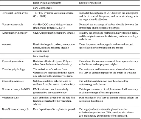
Table 1. Summary of main Earth system additions from HadGEM1 to HadGEM2-ES.
Earth System components Reason for inclusion
New Components
Terrestrial Carbon cycle TRIFFID dynamic vegetation scheme (Cox, 2001)
To model the exchange of CO2between the atmosphere and the terrestrial biosphere, and to model changes in the vegetation distribution.
Ocean carbon cycle diat-HadOCC ocean biology scheme
(Palmer and Totterdell, 2001)
To model the exchange of carbon dioxide between the atmosphere and the oceanic biosphere
Atmospheric Chemistry UKCA tropospheric chemistry scheme To allow the ozone and methane radiative forcing fields, and the sulphate oxidant fields to vary with meteorology and climate
Aerosols Fossil-fuel organic carbon, ammonium
nitrate, dust and biogenic organic aerosols added
These important anthropogenic and natural aerosol species are now represented in the model
New couplings
Chemistry-radiation Radiative effects of O3and CH4are taken from the interactive chemistry
This allows the concentrations of these species to vary with climate and tropopause heights.
Chemistry-hydrology The emissions of methane from wetlands are supplied from the hydrol-ogy scheme to the chemistry scheme.
The emissions and hence concentrations of methane will vary as climate impacts on the extent of wetlands
Chemistry-Aerosols Sulphate oxidation scheme takes its oxidants from the interactive chemistry.
The sulphur oxidation will now be affected by meteorology and climate
Ocean carbon cycle-DMS DMS emission now interactively generated by the ocean biology
This important source of sulphate aerosol will now vary as climate change affects the plankton
Vegetation-Dust Dust emissions depend on the bare soil
fraction generated by the vegetation scheme
Dust production will vary as climate change affects the vegetation distribution
Dust-Ocean carbon cycle Dust deposition affects plankton growth The supply of nutrients to the plankton varies with the dust production. This coupling also allows geo-engineering experiments to be simulated.
2.1 Underlying physical model
The physical model configuration is derived from the HadGEM1 climate model (Johns et al., 2006 and references therein) with improvements as discussed in The HadGEM2 Development Team (2011) and Martin et al. (2010), and is only described briefly here. The atmospheric component uses a horizontal resolution of 1.25◦ × 1.875◦ in latitude and longitude with 38 layers in the vertical extending to over 39 km in height. The oceanic component uses a latitude– longitude grid with a zonal resolution of 1◦everywhere and meridional resolution of 1◦between the poles and 30◦
lati-tude, from which it increases smoothly to 1/3◦at the equator.
It has 40 unevenly spaced levels in the vertical.
The addition of Earth system components to the climate model introduces more stringent criteria on the physical
per-formance. For instance, the existence of biases in temper-ature or precipitation on the regional scale need not detract from a climate model’s ability to simulate future changes in climate; however such biases can seriously affect the ability of the Earth system model to simulate reasonable vegetation distributions in these areas. Hence a focus for the develop-ment of the physical components of HadGEM2 was improv-ing the surface climate, as well as other outstandimprov-ing errors such as El Ni˜no Southern Oscillation (ENSO) and tropical climate. Details of the major developments to the physical basis of the HadGEM2 model family are described in Martin et al. (2010) and The HadGEM2 Development Team (2011). 2.2 Land surface exchange scheme
al., 2011; Clark et al., 2011) is derived. This was targeted for development since surface exchange directly influences the vegetation scheme and the terrestrial carbon cycle. Even without land carbon-climate feedbacks, these changes im-prove the land-surface exchange since water loss through leaves (transpiration) and carbon gain (GPP, gross primary productivity) are intimately linked through the leaf stomatal conductance.
There is an improved treatment of penetration of light through the canopy (Mercado et al., 2007). This involves explicit description of light interception for different canopy levels, which consequently allows a multilayer approach to scaling from leaf to canopy level photosynthesis. The multi-layer approach has been evaluated against eddy-correlation data at a temperate conifer forest (Jogireddy et al., 2006) and at a tropical broad-leaved rainforest site (Mercado et al., 2007), and these studies demonstrated the improved model performance with the multi-layer approach compared with the standard big-leaf approach. The original MOSES II scheme removed excess water by adding it straight into the surface runoff if the top soil level was saturated. In HadGEM2 this is modified to add this into the downward moisture flux in order to retain soil moisture better (Martin et al., 2010).
Lakes in MOSES II do not vary with climate, so the areas remain constant. In HadGEM1 evaporation from lakes was therefore a net source of water into the climate system. In HadGEM2 this evaporation now depletes the soil moisture. It would have been desirable to take this from the surface grid squares containing the lake, but this often led to unacceptably low soil moisture levels. As a compromise, the global lake evaporation flux is calculated and removed evenly from the deep soil moisture over the whole land surface (providing the soil moisture content is greater than the wilting point in the grid box). This water conservation is necessary to diagnose trends in sea level. Precipitation falling onto a grid square adds to the soil moisture regardless of the lake fraction in that grid square, thus always conserving water.
2.3 Hydrology
A large-scale hydrology module (LSH) has been introduced into HadGEM2 in order to improve the soil moisture, and hence the vegetation distribution, and provide additional functionality such as simulation of wetland area required for interactive methane emissions. LSH (Clark and Gedney, 2008; Gedney and Cox, 2003) is based on the TOPMODEL approach (Beven and Kirkby, 1979) whereby soil moisture and runoff are affected by local topography as well as me-teorology, vegetation and soil properties. In the standard scheme (Essery et al., 2003) water was lost out of the bottom of the soil column through gravitational drainage. In LSH the hydraulic conductivity decreases with depth below the root zone allowing a saturated zone to form. Water is lost through lateral sub-surface flow within this saturated zone. Hence
LSH tends to produce more soil moisture in the deeper lay-ers especially when there is relatively little topography (less lateral flow) and when there is partial freezing. In the stan-dard scheme under conditions of partial freezing deep in the soil the unfrozen soil moisture above is lowered. This is be-cause gravitational drainage tends to lead to a small vertical gradient in unfrozen soil moisture. Hence the unfrozen soil moisture contents in the shallower layers are all effectively limited by the extent of soil moisture freezing in the deep layer.
A sub-grid distribution of soil moisture and water table can be inferred from the sub-grid scale distribution in topog-raphy and mean soil moisture. This allows the calculation of partial inundation within each grid box, enhancing surface runoff. The estimate of inundation extent can also be used to diagnose a wetland fraction for calculating interactive wet-land methane emissions (Gedney et al., 2004), for use by the chemistry scheme (Sect. 2.6). The wetland methane scheme requires a soil carbon content. This can be taken from the interactively derived values (Sect. 2.7). However, if anthro-pogenic land use changes are imposed (such as in the stan-dard CMIP5 protocol), carbon can be added to or from the most labile soil carbon pool (see Sect. 2.7). This induces un-realistic changes in wetland methane emissions and hence in that case a soil carbon climatology needs to be used to drive the emissions. Feedbacks associated with changes in soil car-bon, such as due to CO2fertilisation (van Groenigen et al.,
2011) are then not captured.
As in HadCM3, the accumulation of frozen water on the permanent ice sheets is never returned to the freshwater cy-cle; that is, there is no representation of icebergs calving off ice shelves. To counterbalance these sinks in the global an-nual mean freshwater budget a freshwater flux field is applied to the ocean, with a pattern the same as that calibrated for HadCM3 but interpolated to the HadGEM2 ocean grid. Be-cause there is no dynamic ice sheet modelling in HadGEM2 this calving flux does not vary with climate. Therefore if pre-cipitation over ice sheets changes with time this will add or subtract from the snow depth and decrease or increase sea level.
The freshwater fluxes are shown in Fig. 1. The scale used here is Sverdrup (Sv) which corresponds to 106m3s−1or a change in sea level of∼10 m per century. With the changes made to the conservation here and in Sects. 2.2 and 2.4, the fluxes are close to being in equilibrium. The exception to this is the atmosphere. The apparent imbalance in the atmosphere has been traced to a subtle difference between the diagnosed precipitation and the water removed from the atmosphere. 2.4 River model
Fig. 1. Freshwater fluxes in HadGEM2 in Sv (106m3s−1) averaged over 10 yr of the model control run (pre-industrial conditions). Values inside the boxes are the differences between the flow in and out of each box.
the atmosphere or the land surface model, necessitating additional coupling to transfer the runoff fluxes and inte-grated river flows. The inteinte-grated river flows are deposited at predefined coastal outflow points on the atmosphere grid and then passed to the ocean model as a surface freshwater flux term. Errors in the formulation of this coupling led to a lack of water conservation in the HadGEM1 model. An additional loss of water was caused where rivers terminated in inland basins rather than at the coasts. In HadGEM2 this water is now added to the soil moisture at the location of the inland basin until this grid point becomes saturated. For sat-urated basins, water conservation is forced to be maintained by scaling the total coastal outflow.
2.5 Aerosols
Eight aerosol species are now available in HadGEM2. They are ammonium sulphate, ammonium nitrate, fossil-fuel black carbon, fossil-fuel organic carbon, mineral dust, biomass-burning, sea salt and biogenic aerosols. The latter two are not transported but are diagnosed or provided as a climatol-ogy. Aerosols scatter and absorb solar and terrestrial radi-ation (direct effect), and provide the cloud droplet number (indirect effects). The aerosols are coupled with other com-ponents of the model, such as the vegetation scheme and the ocean model.
The nitrate, fossil-fuel organic carbon and biogenic aerosols are new to HadGEM2. The biogenic aerosol cli-matology was found to reduce the continental warm bias
thus improving the vegetation distribution (see Sect. 3.2 and Martin et al., 2010). Changes to the aerosol scheme since HadGEM1 are described in detail in Bellouin et al. (2011). The nitrate aerosols were added after the main model de-velopment and are not included in the CMIP5 integrations (Jones et al., 2011). Nitrate aerosols can only be included if the interactive tropospheric chemistry is used. All other species can be included without tropospheric chemistry.
Important couplings that have been introduced into HadGEM2 are the provision of the oxidants that convert SO2
and DMS to sulphate and the provision of HNO3as a
precur-sor for nitrate aerosols. These sulphur oxidants (OH, H2O2,
HO2 and O3)can be provided as climatological fields (the
oxidation by O3 is new to HadGEM2), or taken from the
interactive tropospheric chemistry scheme. The interactive coupling is important to simulate the changes in oxidation rates with climate change, and with the change in reactive gas emissions. It also ensures that the oxidant concentrations are consistent with the model meteorological fields. Modelled sulphate concentrations obtained with interactively simulated oxidants have been found to compare with observations at least as favourably as those obtained with prescribed oxi-dants. The nitric acid from the interactive chemistry gen-erates ammonium nitrate aerosol with any remaining ammo-nium ions after reaction with sulphate. The sulphate and ni-trate schemes deplete H2O2 and HNO3from the gas-phase
The facility to run the aerosol scheme with prescribed oxidants is still available for model configurations where aerosols, but not gas phase chemistry are required, such as the physics only HadGEM2-AO (HadGEM2 Development team, 2011).
Mineral dust is a new species added to HadGEM2 and is important for its biogeochemical feedbacks. The dust model in HadGEM2 is based on Woodward (2001), but with sig-nificant improvements to the emission scheme (Woodward, 2011). Calculation of dust emission is based on the widely-used formulation of Marticorena and Bergametti (1995) for a horizontal flux size range of 0.03 to 1000 µm radius. Thresh-old friction velocity is obtained from BagnThresh-old (1941) and the soil moisture dependence is based on Fecan et al. (1999). The vertical flux is calculated in 6 bins up to 30 µm radius. Dust affects both shortwave and longwave radiative fluxes, using radiative properties from Balkanski et al. (2007). It is removed from the atmosphere by both dry and wet deposi-tion processes, providing a source of iron to phytoplankton and thus potentially affecting the carbon cycle.
Dust is only emitted from the bare soil fraction of a grid-box, which in the Earth system configuration is calculated by the TRIFFID interactive vegetation scheme. This provides the coupling between vegetation and dust which is an impor-tant component of the biogeochemical feedback mechanisms which this model is designed to simulate. Inevitably, model simulated bare soil fraction is less realistic than the climatol-ogy and this has an undesirable impact on dust production, exacerbated by the increase in wind speed and drying of soil associated with loss of vegetation. In order to limit unreal-istic source areas and so minimise this effect, whilst main-taining a sensitivity to climate-induced vegetation change, a preferential source term (Ginoux, 2001) has been introduced to limit dust emissions to areas of topographic depression. 2.6 Tropospheric chemistry
The atmospheric chemistry component of HadGEM2 is a configuration of the UKCA model (UK Chemistry and Aerosols; O’Connor et al., 2011) which includes tropo-spheric NOx-HOx-CH4-CO chemistry along with some
rep-resentation of non-methane hydrocarbons similar to the TOMCAT scheme (Zeng and Pyle, 2003). The 26 chemical tracers are included in the same manner as other model trac-ers. The chemical emissions from all anthropogenic sources, and most natural sources (including non-wetland methane), are provided as external forcing data (Jones et al., 2011). In-teractive lightning emissions of NOxare included according
to Price and Rind (1993). Photolysis rates are calculated offline in the Cambridge 2-D model (Law and Pyle, 1993). Dry deposition is an adaptation of the Wesely (1989) scheme as implemented in the STOCHEM model (Sanderson et al., 2006). A complete suite of tracer and chemical diagnos-tics has also been included. As the chemical scheme does not take account of halogen chemistry relevant to the
strato-90S 45S
0 45N
90N
Latitude
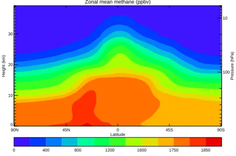
Zonal mean methane (ppbv)
0 400 800 1200 1600 1750 1850
100 10
Pressure (hPa)
0 10 20 30
Height (km)
Fig. 2. Annually average zonal mean methane concentrations gen-erated by the HadGEM2 chemistry driven with 2005 emissions of methane and ozone precursors from Jones et al. (2011).
sphere, stratospheric ozone concentrations are prescribed ac-cording to climatology from the CMIP5 database from 3 levels (3–5 km) above the tropopause. Methane loss in the stratosphere is parameterised with a 60 day decay time in the top three layers (above 28 km).
The motivation for implementing a tropospheric chem-istry, but not a stratospheric one, was based largely on the focus on biogeochemical couplings. These involve the oxi-dation of SO2and DMS to form sulphate aerosol, the
emis-sions of methane from wetlands and the radiative impacts of tropospheric ozone and methane. Stratospheric chemistry would not be useful unless the model top were raised and the vertical resolution in the stratospheric increased, both of which would slow the model. Interactive chemistry is com-putationally very expensive, due both to the advection of the many tracers and the integration of the chemical equations. For this reason only a simple tropospheric chemistry scheme could be afforded for centennial-scale climate integrations.
The UKCA interactive chemistry in HadGEM2 takes methane emissions from wetlands generated by the large-scale hydrology scheme (Sect. 2.3). The overall scaling was chosen to give emissions of approximately 130 Tg methane per year under pre-industrial conditions.
The interactive gas-phase chemistry provides oxidants (HO2, H2O2, and O3)and nitric acid (HNO3)to the aerosol
scheme, which in turn depletes H2O2 and HNO3 from the
2.7 Terrestrial carbon cycle
The terrestrial carbon cycle component of HadGEM2 is made up of the TRIFFID dynamic vegetation model (Cox, 2001; Clark et al., 2011) and an implementation of the RothC soil carbon model (Coleman and Jenkinson, 1999). The TRIFFID vegetation scheme had been used in a configura-tion from a previous generaconfigura-tion of Hadley Centre models (HadCM3LC). It simulates phenology, growth and compe-tition of 5 plant functional types (broad-leaved and needle-leaved trees, C3 and C4 grasses and shrubs).
An agricultural mask is applied to prevent tree and shrub growth in agricultural regions. This mask can vary in time in transient simulations allowing HadGEM2 to represent both biophysical and biogeochemical impacts of land use change. When the mask is applied to areas previously occupied by trees and shrubs, these areas are converted to bare soil and the carbon previously stored in the vegetation is moved to the most labile soil carbon pool. While there is no explicit crop plant functional type, these new bare soil areas can be taken over by the C3 and C4 grasses. There is no irrigation or harvesting applied to the grasses.
A primary reason for including a dynamic vegetation model in HadGEM2 is to simulate the global distribution of fluxes and stores of carbon. Organic carbon is stored in the soil when dead litter falls from vegetation, either as dropped leaves or branches or when whole plants die. It is returned to the atmosphere as heterotrophic respiration when soil or-ganic matter is decomposed by microbes. In HadGEM2 we have implemented the 4-pool RothC soil carbon model (Coleman and Jenkinson, 1999) which simulates differen-tiated turnover times of four different pools of soil carbon ranging from easily decomposable plant matter to relatively resistant humus. Multi-pool soil carbon dynamics have been shown to affect the transient response of soil carbon to cli-mate change (Jones et al., 2005). Although each RothC pool currently has the same sensitivity to soil temperatures and moisture there is the ability to allow the model to enable different sensitivities for each pool as suggested by Davidson and Janssens (2006). Note that this model is not designed to simulate the large carbon accumulations in organic peat soils, or the stocks and dynamics of organic matter in permafrost.
Global carbon stores are determined by the fluxes of car-bon into and out of the vegetation/soil system. The fluxes “in” are due to vegetation productivity (supplied to TRIFFID from the surface exchange scheme), and the fluxes “out” due to vegetation and soil respiration. Productivity is frequently expressed as gross primary production (GPP) which is the total carbon uptake by photosynthesis, and net primary pro-duction (NPP) which is the difference between GPP and plant respiration (carbon released by the plant’s metabolism), pa-rameterised as the sum of the growth and maintenance terms. The carbon cycle is closed by the release of soil respiration – decomposition of dead organic matter. In the absence of fires or time-varying land use, the net flux (net ecosystem
ex-change, NEE, or net ecosystem productivity, NEP) is there-fore given by GPP-total respiration.
A comprehensive calibration of the terrestrial ecosystem parameters has been undertaken to improve the carbon fluxes compared to HadCM3LC, some of which have been de-scribed in Sect. 2.2. The Q10 temperature response
func-tion of soil heterotrophs was kept from HadCM3LC, rather than using the generic function in RothC (which leads to too low soil respiration in winter). In addition the soil respira-tion is now driven by soil temperatures from the second soil layer instead of the first layer as in HadCM3LC, as most of the decomposable soil carbon would be on average at this depth. This leads to a smaller seasonal cycle in soil temper-atures, and thus reduced seasonality in soil respiration with-out affecting long-timescale sensitivity to temperature. The response of soil respiration to moisture is represented by the total soil moisture (frozen plus unfrozen), compensating for a cold bias in high latitude winter soil temperatures (due to insufficient insulation of soil under snow (Wiltshire, 2006)). Seasonality in leaf phenology of temperate ecosystems, and thus seasonal plant productivity, is improved by delaying the onset of the growing season relative to HadCM3LC using a 5◦C growing degree base for the deciduous vegetation
phe-nology, as used in Sitch et al. (2003). This contributes to an improved simulation of photosynthesis. The above changes are described in more detail in Cadule et al. (2010).
While the transport of atmospheric tracers in HadGEM2 is designed to be conservative, the conservation is not per-fect and in centennial scale simulations this non-conservation becomes significant. This has been addressed by employ-ing an explicit “mass fixer” which calculates a global scal-ing of CO2 to ensure that the change in the global
atmo-spheric mean mass mixing ratio of CO2 in the atmosphere
matches the total flux of CO2into or out of the atmosphere
each timestep (Corbin and Law, 2010).
2.8 Ocean carbon cycle
The ocean biogeochemistry component in HadGEM2 vides the ocean component of the carbon cycle and the pro-vision of di-methyl sulphide (DMS) emissions from phyto-plankton. It consists of an ecosystem model and related sub-models for seawater carbon chemistry and the air-sea trans-port of CO2, the cycling of iron supplied by atmospheric
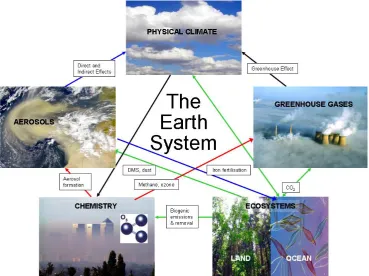
Fig. 3. Earth system couplings feedbacks.
requirement for silicate) and allows an improved representa-tion of the biological pump and of DMS producrepresenta-tion.
Iron, carbon, dissolved inorganic nitrogen and silicate are transported as three dimensional tracers in the ocean. Iron is now recognised as an important micro-nutrient for phy-toplankton, which can limit growth in some areas of the ocean (including the Southern Ocean and parts of the North and Equatorial Pacific). In many ocean areas iron found in the surface waters has mainly been supplied by atmospheric dust deposition (the Southern Ocean is an exception), and al-though utilisation by phytoplankton can be a temporary sink this iron is quickly recycled and the long-term removal pro-cess is transfer to the sediments via adsorption onto mineral particles. Modelling iron cycling in the ocean allows us to examine possible climate feedbacks whereby increased dust production improves iron availability in the ocean, strength-ening the biological pump and increasing the uptake of CO2
by the ocean.
DMS, which is a significant source of sulphate aerosol over the oceans, is produced within Diat-HadOCC using the parameterisation of Simo and Dachs (2002) as described in Halloran et al. (2010). This scheme relates the DMS production to surface water chlorophyll concentrations and the depth of the corresponding mixed layer.
3 Developing the coupled model 3.1 Couplings in HadGEM2
One of the prime motivations for incorporating Earth system processes, which cannot be achieved with offline modelling, is to include Earth system couplings (Fig. 3). Combinations of these couplings form biogeochemical feedback loops. The couplings take place every dynamical timestep (30 min in this configuration) within the land-atmosphere system, ex-cept for those involving radiation which take place every 3 h. Coupling between the ocean and the atmosphere is on a daily timescale. The vegetation distributions are updated every 10 days. All components are driven by the physical climate.
The gas-phase chemistry is coupled to the aerosol scheme through the provision of concentrations of OH, H2O2and O3
for the oxidation of SO2and DMS, and is coupled to the
ra-diation scheme through the provision of three dimensional concentrations of O3and CH4. The aerosols are coupled to
the cloud microphysics and the radiation scheme. The dust deposition is coupled to the ocean biogeochemistry and sup-plies iron nutrient. There is no impact of the aerosols on the chemistry, e.g. through heterogeneous reactions or effect on the photolysis rates, except that the aqueous-phase SO2
oxi-dation depletes H2O2in the chemistry and the nitrate aerosol
The land ecosystems determine the exchange of CO2
be-tween the land and the atmosphere. They are coupled to the physical climate through the vegetation distribution and leaf area index which affects the surface albedo, the stomatal con-ductance which determines the evapotranspiration flux, and the roughness length which affects the surface wind and mo-mentum transport. The vegetation cover controls the dust emissions, and the wetland model supplies methane emis-sions to the atmospheric chemistry. Surface removal (dry de-position) of gas-phase chemical species and aqueous-phase aerosols also depends on the vegetation cover and stomatal conductance. Other emissions of trace gases and aerosols from the terrestrial biosphere such as from vegetation, soils and fires are not considered.
As well as determining the ocean-atmosphere exchange of CO2, the ocean biogeochemistry scheme provides a flux of
DMS into the atmosphere, thus providing a source of sul-phate aerosol precursor.
Many feedback loops can be constructed from Fig. 3, and hence can be examined in HadGEM2 configurations. Nu-merous studies (e.g. Friedlingstein et al., 2006; Sitch et al., 2008) have looked at the loop from the climate impacts on ecosystems to the CO2 concentrations and back to climate.
The Charlson, Lovelock, Andreae, Warren (CLAW) hypoth-esis (Charlson et al., 1987) described a loop from climate to ocean biogeochemistry, sulphate aerosols, cloud micro-physics and to climate. In HadGEM2-ES this can be ex-tended by starting the CLAW loop by following the coupling from climate to terrestrial vegetation, dust emissions, iron de-position and the fertilisation of the ocean biogeochemistry.
Future experiments will quantify the individual feedback pathways through breaking coupling loops in specific places by replacing exchanged quantities with prescribed fields. 3.2 Development and spin up
When combining multiply connected model components there are numerous possibilities for biases in one place to disrupt the evaluation in another. In extreme cases this could lead to runaway feedbacks where components drive each other further and further from a realistic representation of the observed state. In the HadGEM2 development process, each Earth system component was initially developed sepa-rately from the others by being coupled only to the physical atmosphere or ocean, with the other components represented by climatological data fields. Only when all the individual components proved to be stable and realistic were these data fields replaced by interactive couplings.
An example of this was the interaction between the surface climate and the dynamic vegetation. The TRIFFID scheme was initially tested in the HadGEM1 physical climate model. The model had a very low soil moisture (compared the previ-ous generation of Met Office Hadley Centre models such as HadCM3LC) in the summertime in the centres of the ern continents (central and northern Asia., central and
north-ern North America). This dryness reduced the growth of veg-etation; however with less vegetation the soils dried out fur-ther. This process eventually led to the decline of all vegeta-tion in these regions and extreme summer temperatures and dryness.
The increase in the summertime continental soil moisture was one of the improvements made to the physical model in the development from HadGEM1 to HadGEM2 (Martin et al., 2010). In parallel the TRIFFID model was developed in a configuration driven by observed meteorology where im-provements were made to give a more realistic tolerance to arid conditions. Before being finally combined, TRIFFID was driven offline by meteorology from the HadGEM2 phys-ical model. This ensured the final coupled configuration was stable.
The components were spun up to 1860 climate conditions, which we refer to as “pre-industrial”, by imposing emissions or concentrations of gases and aerosols as specified by the CMIP5 project (see Jones et al., 2011). The species for which concentrations were imposed are N2O, halocarbons
and stratospheric ozone. We assumed the climate system to be approximately in equilibrium at this time. The Earth system components with long timescales (decade or more) are the ocean physical and nutrient variables, the vegetation distribution, the soil carbon content and the methane concen-trations. The deep ocean circulation operates on timescales of millennia or tens of millennia. In practice, we chose to spin up to a state where drifts over the length of an expected model experiment (around 300 yr) were small. Drifts can be accounted for in experimental setups by running a control integration parallel to the experiment.
The TRIFFID vegetation scheme has a fast spin up mode in which it can use an implicit timestep to take 100 yr jumps every 3 model years. After the physical and vegetation im-provements described above, a near-stable distribution in the coupled system is achieved after 12 model years (equiva-lent to 400 vegetation years) for 1860 conditions. The fast spin up of vegetation cover is not fully successful at spinning up the soil carbon stores, because sub-annual fluctuations in the litter inputs are of comparable magnitude to changes in the small, rapid-turnover decomposable plant material pool which subsequently affects the long-lived humified organic matter pool. Hence, an offline spin-up of the soil carbon model was carried out to spin up the least labile soil carbon store of humified organic matter (e-folding time of around 50 yr). Using monthly mean diagnostics of litter inputs and rate modifying factors the soil carbon model was run offline for 2000 yr until all the pools had reached steady state. A fi-nal equilibration of vegetation cover and soil carbon storage was then achieved by running the model with TRIFFID in its normal, real-time mode for a further 10–20 yr with fixed at-mospheric CO2(286 ppm). This distribution is evaluated in
Atm surface CO2
0 50 100 150 200 250 300
year 270
275 280 285 290 295 300
ppm
Land Carbon
0 50 100 150 200 250 300
year 1550
1560 1570 1580 1590 1600
GtC
Ocean Primary Production
0 50 100 150 200 250 300
year 30
32 34 36 38 40
GtC/yr
air-to-sea CO2 flux
0 50 100 150 200 250 300
year -0.6
-0.4 -0.2 0.0 0.2 0.4 0.6
GtC/yr
Fig. 4. Atmospheric CO2, land carbon store, ocean primary pro-ductivity and the air to sea CO2flux from 280 yr of the HadGEM2 control integration under 1860 conditions.
To ensure stability when all Earth system components were combined, this over predicted dust was used in the spin up of the ocean biogeochemistry.
The physical ocean was initialised from a control run from the previous (HadGEM1) climate model (Johns et al., 2006) with biogeochemical fields from HadCM3LC (C and N) or Garcia et al. (2010) for Si. Fe was initialised to a constant value. The ocean was spun up first for 400 yr in an ocean-only configuration with forcings (meteorology, atmospheric CO2, dust input) provided as external driving fields. After
this time the upper ocean nutrients and vertically integrated primary productivity had stabilised. The ocean was coupled back to the atmosphere and the composition fields (DMS, dust). With the components of the carbon cycle now equili-brated, the constraint on the atmospheric CO2concentrations
could be removed and the model allowed to reach its own equilibrium.
Figure 4 shows the carbon cycle variables from 280 yr of the control integration following the spin up. This uses continuous 1860 forcing conditions. Trends are very small, particularly in the atmospheric CO2concentrations, showing
that the system has successfully spun up. There is a slight in-crease in the land carbon of about 5 Gt(C) after 280 yr. This would correspond roughly to a decrease in the atmospheric concentration of 0.01 ppm per yr which is negligible com-pared to any anthropogenically-forced experiments. The air to sea CO2flux is close to zero, confirming that the terrestrial
and oceanic carbon fluxes have equilibrated.
Of the gas-phase and aerosol chemical constituents, only methane has a long enough lifetime to require spinning up. For the core CMIP5 control run (Jones et al., 2011), methane surface concentrations were specified rather than interactively calculated so little spin up was needed. How-ever for the model to be suitable for further investigations
Fig. 5. Methane concentrations from the spin up of the chemistry components under 1860 conditions.
180 90W 0 90E
90S 45S 0 45N 90N
JJA obs wetland (Prigent)
0.025 0.05 0.1 0.2 0.3 0.4
180 90W 0 90E
90S 45S 0 45N 90N
JJA Modelled wetland
0.025 0.05 0.1 0.2 0.3 0.4
180 90W 0 90E
90S 45S 0 45N 90N
JJA obs wetland (Prigent)
0.025 0.05 0.1 0.2 0.3 0.4
180 90W 0 90E
90S 45S 0 45N 90N
JJA Modelled wetland
0.025 0.05 0.1 0.2 0.3 0.4
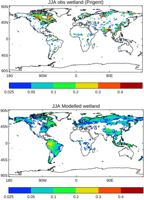
Fig. 6. June-July-August average inundation fraction: (a) satellite observations (Prigent et al., 2001, b) HadGEM2 model.
180 90W 0 90E 180 90S
45S 0 45N 90N
Coastal River Discharge - Observations (Sv)
5e-4 0.002 0.01 0.05 0.2
180 90W 0 90E 180
90S 45S 0 45N 90N
Coastal River Discharge - HadGEM2-ES (Sv)
5e-4 0.002 0.01 0.05 0.2
Fig. 7. Mean annual (1948–2004) discharge (Sv) from 4◦latitude by 5◦longitude coastal box estimated from available gauge records and reconstructed river flow (Dai et al., 2009) and simulated discharge from HadGEM2.
was 59 Tg yr−1, oceans and termites totalled 45 Tg yr−1, so the wetland component was adjusted to give the required to-tal (237 Tg yr−1). This was run for 15 yr to verify that the methane concentrations were close to the observed 805 ppb (see Fig. 5).
4 Evaluation of components
The long-timescale Earth system components (terrestrial and ocean carbon cycles) were developed under 1860 conditions as described in Sect. 3, which limited the comparisons that could be carried out at that stage. The model has now been run through the historical period (Jones et al., 2011) thus al-lowing comparison with present day observations.
The aerosols and chemistry equilibrate on sufficiently short timescales that they could be developed and evaluated in atmosphere-only configurations of the model forced with AMIP sea surface temperatures and sea ice (Gates et al., 1999).
Martin et al. (2010) evaluates the impacts of the devel-opments to the physical model. Of particular note are the improvements to the northern summertime surface tempera-tures and the net primary productivity (their Figs. 13 and 17). Further physical evaluation is available in The HadGEM2 Development Team (2011).
4.1 Land surface hydrology and the river model
The land surface hydrology model provides runoff for the river flow model and also predicts inundation area for use in the wetland emission scheme (Sect. 4.3). Figure 6 compares the modelled northern hemisphere summer inundation frac-tion against that derived from an Earth observafrac-tions prod-uct (Prigent et al., 2001). The model distribution is much smoother than the satellite product which has very localised areas with high inundation fractions. Some inundation ar-eas such as central Canada seem to be missing from the model. The model significantly over-estimates inundation
extent over the Amazon basin. This is probably due to poor data on the underlying rock topography in this region as used in the driving topographic dataset.
Rivers provide significant freshwater input to the oceans thereby forcing the oceans regionally through changes to density. The inclusion of the TRIP river flow model allows the inclusion of this regional ocean forcing, which is an im-portant component of both Earth system and atmosphere-ocean models. The total HadGEM2-ES simulated discharge to the oceans is 1.07 Sv, within the observational range of 1.035 to 1.27 Sv (Dai and Trenberth, 2002) but tending to the low side. Figure 7 compares the simulated regional dis-charge from HadGEM2-ES and an observational dataset of ocean discharge from Dai et al. (2009). HadGEM2-ES sim-ulates the point of river discharge in a slightly different loca-tion to the observaloca-tions due to the smoothed land-sea mask of the ocean model. However, the major rivers such as the Amazon, Ganges/Brahmaputra and Mississippi are all well simulated.
4.2 Aerosols
The improved aerosols in HadGEM2 have been extensively evaluated in Bellouin et al. (2007, 2011) and The HadGEM2 Development Team (2011). Here we focus specifically on the biogeochemical couplings between aerosols and the oceanic and terrestrial ecosystems through emissions of DMS and mineral dust.
DMS concentrations at Amsterdam Island
J F M A M J J A S O N D
Month 0.0
0.2 0.4 0.6 0.8 1.0
μ
g[S]/m
3
Observations HadGEM2-AO HadGEM2-ES
DMS concentrations at Dumont d’Urville
J F M A M J J A S O N D
Month 0.0
0.2 0.4 0.6 0.8 1.0
μ
g[S]/m
3
Observations HadGEM2-AO HadGEM2-ES
DMS concentrations at Cape Grim
J F M A M J J A S O N D
Month 0.0
0.2 0.4 0.6 0.8 1.0
μ
g[S]/m
3
Observations HadGEM2-AO HadGEM2-ES
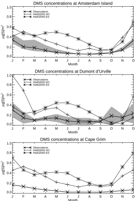
Fig. 8. Comparison of DMS concentrations in the southern mid and high latitudes with the HadGEM2 simulations; with (HadGEM2-ES) and without (HadGEM2-AO) interactive ocean biology. Ob-servations are from Ayers et al. (1991), Jordain et al. (2001) and Nguyen et al. (1992). For Amsterdam Island the shaded area spans the 5–95 % range of the observations, for Dumont d’Urville it spans the±2 standard deviation range. For Cape Grim only the mean concentrations are available.
to over predict the austral winter atmospheric concentrations compared to using the prescribed sea water concentrations. This is in spite of the good comparison between the sim-ulated and observed ocean concentrations (as seen later in Sect. 4.5 and Fig. 21). This suggests that there may be re-gional differences in the emissions. At the Antarctic station of Dumont d’Urville, the interactive scheme does better at simulating the austral summer concentrations. As seen in Fig. 21, the Kettle et al. (1999) climatology used to prescribe DMS overestimates these concentrations.
Dust production is highly sensitive to various atmospheric and surface variables, and the introduction and coupling to-gether of new biogeochemical components – particularly teractive vegetation – in the Earth system model will in-evitably lead to changes in these variables, not all of which
180 90W 0 90E 180
90S 45S 0 45N 90N
Dust load (mg m-2)
0 20 100 500 2000 1e+4
Fig. 9. Modelled decadal mean dust load in HadGEM2-ES for 1991–2000.
Fig. 10. Comparison of modelled (HadGEM2-ES) and observed near surface dust concentrations and total aerosol optical depths (AODs) at 440 nm. Observed optical depths are from AERONET stations in dust-dominated regions and concentrations from stations of the University of Miami network (with thanks to J. M. Prospero and D. L. Savoie). Symbols indicate: crosses – AODs, stars – At-lantic concentrations, squares – N Pacific concentrations, triangles – S Pacific concentrations, diamonds – Southern Ocean concentra-tions.
180 90W 0 90E 180 90S
45S 0 45N 90N
Difference in dust load (mg m-2 )
-1000 -200 -50 -10 10 50 200 1000
180 90W 0 90E 180
90S 45S 0 45N 90N
Difference in bare soil fraction
-1 -0.8 -0.6 -0.4 -0.2 0.2 0.4 0.6 0.8 1
180 90W 0 90E 180
90S 45S 0 45N 90N
-1000 -200 -50 -10 10 50 200 1000
180 90W 0 90E 180
90S 45S 0 45N
90N Difference in bare soil fraction
-1 -0.8 -0.6 -0.4 -0.2 0.2 0.4 0.6 0.8 1
Fig. 11. Differences in dust load (above) and bare soil fraction (below) between HadGEM2-ES and an atmosphere-only simulation (HadGEM2-A) forced by AMIP SSTs, using fixed vegetation from IGBP. Values are decadal means 1991–2000.
sources, though concentrations in the Pacific are somewhat too high. This is due to excess dust from areas where an un-realistically high bare-soil fraction, combined with the con-sequent drying of the surface and increase in wind speed, have caused anomalous emissions, particularly in Australia, India and the Sahel (Fig. 11). Despite these limitations, the global dust load is sufficiently well represented for the pur-pose of investigating the biogeochemical feedback processes involving dust.
Interactive emission schemes are unlikely to perform as well as using prescribed emissions. However they allow us to include feedbacks between the biological components and the atmospheric composition, and make predictions of future levels of emissions.
4.3 Evaluation of Chemistry Component of HadGEM2
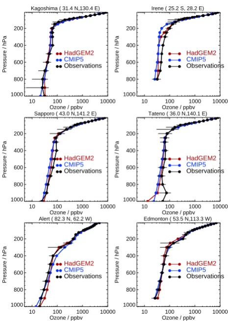
Figure 12 shows comparisons of July vertical ozone pro-files from the HadGEM2 interactive chemistry run compared with the ozone climatology supplied for the CMIP5 project (Lamarque et al., 2010) and climatological observations at a subset of sites from Logan (1999). Data are compared for
Kagoshima ( 31.4 N,130.4 E)
10 100 1000 10000
Ozone / ppbv 1000
800 600 400 200
Pressure / hPa
HadGEM2
CMIP5 Observations
Irene ( 25.2 S, 28.2 E)
10 100 1000 10000
Ozone / ppbv 1000
800 600 400 200
Pressure / hPa
HadGEM2
CMIP5 Observations
Sapporo ( 43.0 N,141.2 E)
10 100 1000 10000
Ozone / ppbv 1000
800 600 400 200
Pressure / hPa
HadGEM2
CMIP5 Observations
Tateno ( 36.0 N,140.1 E)
10 100 1000 10000
Ozone / ppbv 1000
800 600 400 200
Pressure / hPa
HadGEM2
CMIP5 Observations
Alert ( 82.3 N, 62.2 W)
10 100 1000 10000
Ozone / ppbv 1000
800 600 400 200
Pressure / hPa
HadGEM2
CMIP5 Observations
Edmonton ( 53.5 N,113.3 W)
10 100 1000 10000
Ozone / ppbv 1000
800 600 400 200
Pressure / hPa
HadGEM2
CMIP5 Observations
Fig. 12. Comparison of modelled July vertical ozone profiles with climatological observations (black) from Logan 1999), interactive chemistry (red) and the CMIP5 ozone concentrations (blue).
1990–1994 in each case. The HadGEM2 data are taken from a transient run. Note that we used the same anthropogenic emissions of ozone precursors as were used by Lamarque et al. to generate the CMIP5 climatology. The comparison in-dicates that the vertical ozone profiles from HadGEM2 and the CMIP5 datasets compare well with observations. From 3 km above the tropopause, the interactive ozone values are relaxed to the CMIP5 climatology.
The HadGEM2 ozone concentrations near the tropical tropopause are higher than in the CMIP5 climatology due to a lower ozone tropopause in HadGEM2 (diagnosed from the 150 ppb contour). This leads to slightly higher tropical tropopause temperatures when using the interactive ozone.
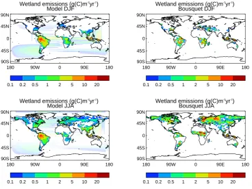
The wetland methane emissions are shown in Fig. 13. As well as the major tropical wetlands, there are significant bo-real emissions during the northern summer. The global total is 137 Gt (CH4)yr−1. 80 % of the emissions are in the tropics
180 90W 0 90E 180 90S
45S 0 45N 90N
Wetland emissions (g(C)m-2
yr-1
) Model DJF
0.1 0.2 0.5 1 2 5 10 20
180 90W 0 90E 180
90S 45S 0 45N 90N
Wetland emissions (g(C)m-2
yr-1
) Bousquet DJF
0.1 0.2 0.5 1 2 5 10 20
180 90W 0 90E 180
90S 45S 0 45N 90N
Wetland emissions (g(C)m-2
yr-1
) Model JJA
0.1 0.2 0.5 1 2 5 10 20
180 90W 0 90E 180
90S 45S 0 45N 90N
Wetland emissions (g(C)m-2
yr-1
) Bousquet JJA
0.1 0.2 0.5 1 2 5 10 20
Fig. 13. Distribution of emissions of methane from wetlands provided to the HadGEM2 chemistry scheme by the large-scale hydrology, compared to those from an inversion study (Bousquet et al., 2006).
90 60 30 0 -30 -60 -90
Latitude 1500
1600 1700 1800 1900 2000
CH
4
/ ppbv
Measurements
HadGEM2-ES
Fig. 14. Comparison of modelled methane concentrations for the 1990s compared with observations from a selection of sites from NOAA ESRL (Dlugokencky et al., 2011).
emissions over Amazonia are due to the over-estimate of the modelled inundation extent (see Sect. 4.1).
The seasonal patterns of the modelled wetland fluxes are compared qualitatively against those of an inversion study (Bousquet et al., 2006) in Fig. 13. It should be noted that the spatial pattern here derives mainly from the data used (Matthews and Fung, 1987) as the prior for the inversion.
The locations of the seasonal maxima for most of the North-ern mid and high latitudes are consistent between the model and the inversion. The differences between modelled and observed inundation areas previously shown in Fig. 6 can also be seen as differences in the wetland methane emissions. The movement of the zone of maximum methane emissions over Central Africa follow similar seasonal patterns. Over S.E. Asia there is considerable disagreement in the magni-tude of natural wetland fluxes. This is likely to be due to difficulties in separating man-made and natural inundation (Chen and Prinn, 2006).
The latitudinal variation in the surface methane concen-tration is shown in Fig. 14, and is compared against sur-face measurements from NOAA ESRL (Dlugokencky et al., 2011). The agreement at the individual sites is reasonable, although the latitudinal gradient is slightly weaker in the model. The methane lifetime for present day (2005) con-ditions is 8.8 yr; in good agreement with previous studies (Stevenson et al., 2006).
4.4 Terrestrial carbon cycle
In the model development stage we evaluated and calibrated the simulation of the terrestrial carbon cycle by HadGEM2 in a pre-industrial control phase, with atmospheric CO2held
Tree cover: IGBP
0.1 0.2 0.4 0.6 0.8 1
Grass/shrub cover: IGBP
0.1 0.2 0.4 0.6 0.8 1
Bare soil: IGBP
0.1 0.2 0.4 0.6 0.8 1
Tree cover: HadGEM2-ES
0.1 0.2 0.4 0.6 0.8 1
Grass/shrub cover: HadGEM2-ES
0.1 0.2 0.4 0.6 0.8 1
Bare soil: HadGEM2-ES
0.1 0.2 0.4 0.6 0.8 1
Tree cover: HadCM3LC
0.1 0.2 0.4 0.6 0.8 1
Grass/shrub cover: HadCM3LC
0.1 0.2 0.4 0.6 0.8 1
Bare soil: HadCM3LC
0.1 0.2 0.4 0.6 0.8 1
Fig. 15. IGBP Climatology and HadGEM2-ES simulation of tree cover (defined as the total of both broadleaf and needleleaf tree), grass, shrub and bare soil.
180 90W 0 90E
90S 45S 0 45N 90N
Soil Carbon: IGBP
0 5 10 15 20 25
180 90W 0 90E
90S 45S 0 45N 90N
Soil Carbon: HadGEM2-ES
0 5 10 15 20 25
180 90W 0 90E
90S 45S 0 45N
90N Soil Carbon: HadCM3LC
0 5 10 15 20 25
60S 30S 0
30N 60N 90N
Latitude 0
5 10 15 20 25
kgC m
-2
IGBP HadGEM2-ES HadCM3LC
0 500 1000 1500 2000 2500 Soil Carbon / GtC
0 200 400 600 800 1000 1200
Vegetetaion Carbon / GtC
Fig. 17. Present day global total soil and vegetation carbon (GtC) from the 11 C4MIP models (black crosses) and HadGEM2-ES (red star) compared with estimated global totals of: biomass (Olson et al., 1985, present 2 central estimates of global vegetation carbon (dashed horizontal lines) and high and low confidence limits – dot-ted); soil carbon (Prentice et al., 2001, state a global estimate of 1350 GtC not including inert soil carbon – dashed vertical line). In the absence of estimated uncertainty range for soil carbon we choose±25 % as a reasonable tolerance (dotted lines).
60S 30S
0 30N
60N 90N
Latitude 0
1•10-8
2•10-8
3•10-8
4•10-8
kgC m
-2 s
-1
Potsdam ±3s.d.
MODIS
Pre-industrial HadGEM2-ES Present day HadGEM2-ES
Fig. 18. Zonal mean distribution of NPP from HadGEM2-ES (pre-industrial simulation in blue, present day simulation in red) com-pared with datasets of global NPP from the Potsdam model database (black) with±3 standard deviations (shaded) and MODIS (Heinsch et al., 2003; black dashed).
simulations for the different parameter combinations in or-der to evaluate the model against present day observations. The main aim is to assess how well the model performs and whether it is fit for purpose as an Earth System model, but we also make use of a comparison against HadCM3LC simula-tions as a benchmark and, where available, some data from the range of C4MIP coupled climate-carbon cycle models (Friedlingstein et al., 2006). Such a comparison is inher-ently imperfect due to the significant changes in the Earth
system over the period 1860-present. Hence we also show here a comparison of the model state with the final parameter setup from a transient historical climate simulation with cli-mate forcings representative of the 20th century implemented as described by Jones et al. (2011). Developing the ter-restrial carbon cycle model within the pre-industrial control phase may lead to some discrepancy between the eventual HadGEM2 present-day simulation and observed datasets. We demonstrate here that the model performance is suffi-ciently good to make HadGEM2 fit for purpose.
4.4.1 Vegetation cover
It is still rare for dynamic vegetation models to be coupled within climate GCMs. In C4MIP only 2 out of the 11 mod-els were GCMs with dynamic vegetation, and both of those had some form of climate correction term such as ocean heat flux adjustment to enable the vegetation simulation to be sufficiently realistic. HadGEM2 dynamically simulates vegetation without a need for any flux-correction to its cli-mate state. The vegetation simulation of HadGEM2 com-pares favourably with observed land cover maps and is gen-erally a little better than that simulated by HadCM3LC. We compare present day conditions from transient simulations of HadCM3LC (as performed for C4MIP; Friedlingstein et al., 2006) and HadGEM2-ES (as performed for CMIP5; Jones et al., 2011) with the observed IGBP climatology (Loveland et al., 2000). Agricultural disturbance is representative of present day.
Figure 15 shows the observed and simulated total tree cover, grass and shrub cover and bare soil. For broadleaf trees (not shown separately) HadGEM2-ES is generally a lit-tle better than HadCM3LC, especially in temperate latitudes where it correctly simulates some coverage in the mixed for-est areas to the southern edge of the boreal forfor-est zone. In the tropics both GCMs have a tendency to simulate too much tropical forest, although this excess is lower in HadGEM2-ES: the latter also has an improved coverage in the north east of Brazil where HadCM3LC has a gap in the forest. For needleleaf trees HadGEM2-ES simulation is similar to that of HadCM3LC. Neither model correctly simulates the area of cold-deciduous larch forest in east Siberia whose phenol-ogy is not well represented in TRIFFID. Overall HadGEM2-ES does a good job at simulating the global distribution of trees.
NEP
0 2 4 6 8 10 12
Month -200
-100 0 100 200
gC m
-2 month
-1
GPP
0 2 4 6 8 10 12
Month 0
100 200 300 400
gC m
-2 month
-1
NPP
0 2 4 6 8 10 12
Month 0
100 200 300 400
gC m
-2 month
-1
Plant Resp.
0 2 4 6 8 10 12
Month 0
100 200 300 400
gC m
-2 month
-1
Soil Resp.
0 2 4 6 8 10 12
Month 0
100 200 300 400
gC m
-2 month
-1
Total Resp.
0 2 4 6 8 10 12
Month 0
100 200 300 400
gC m
-2 month
-1
Obs. HadCM3LC HadGEM2-ES
Fig. 19. Observed and simulated carbon fluxes at Harvard Forest site, USA. HadGEM2-ES (red), HadCM3LC (green). Observations are the mean of 8 yr from AMERIFLUX, .(http://public.ornl.gov/ameriflux/)
Bare soil is diagnosed from the absence of simulated veg-etation. HadGEM2-ES captures the main features of the world’s deserts, and is better than the previous simulation of HadCM3LC except in Australia where it now simulates too great an extent of bare soil. The main tropical deserts are captured as before, but now HadGEM2-ES also simu-lates better representation of bare soil areas in mid-latitudes and the south western USA. As before, the simulated Sa-hara/Sahel boundary is slightly too far south. Along with Australia, there is also too much bare soil in western In-dia in common with HadCM3LC. The presence of too much bare soil in Australia causes problems for the dust emissions scheme.
4.4.2 Simulation of terrestrial carbon stores
Correctly simulating the correct magnitude of global stores of carbon is essential in order to be able to simulate the effect of climate on carbon storage. If the model simulates much too much or too little terrestrial carbon then the impact of climate will be over or under estimated. Jones and Falloon (2009) show the strong relationship between changes in soil organic carbon and the overall magnitude of climate-carbon cycle feedback.
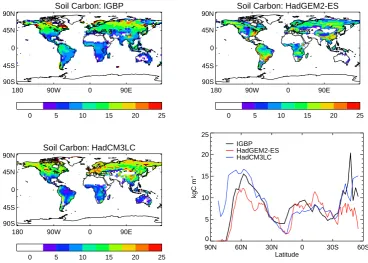
Figure 16 shows the observed (Zinke et al., 1986) and simulated distribution of soil carbon. Both HadGEM2-ES and HadCM3LC models do a reasonable job at represent-ing the main features with HadGEM2-ES improved in the extra-tropics but now over-representing slightly the observed soil carbon in the tropics (especially in Brazil and southern Africa). Insufficient vegetation in Siberia and Australia leads inevitably to too little soil carbon in those regions, which pre-viously had too much.
Global total soil carbon is estimated as about 1500 GtC but with considerable uncertainty (Prentice et al., 2001). HadGEM2-ES simulates 1107 GtC globally for the period 1979–2003, while HadCM3LC simulates 1200 GtC. Consid-ering that about 150 GtC of the observed estimate will be more inert carbon (not represented in our models) and that the models are not yet designed to simulate the large car-bon accumulations in organic peat soils, it may be expected that the simulations underestimate the global total. The range of simulated soil carbon from the 11 C4MIP models is 1040–2210 GtC, so HadGEM2-ES lies comfortably within this range (Fig. 17) although towards the lower end.
90E 180 90W 0 45S
0 45N 90N
Control run: geographical location of histogram bins log(Control run surface chl.)
0.0 0.2 0.4 0.6 0.8 1.0
normalised frequency -4.875 -3.875 -2.875 -1.875 -0.875 0.125
90E 180 90W 0
45S 0 45N
90NSeaWiFs: geographical location of histogram bins
-4.5 -3.75 -3 -2.25 -1.5 -0.75 0 0.75 bin centre log(chlorophyll) mg/m2
log(SeaWiFS surface chl.)
0.0 0.2 0.4 0.6 0.8 1.0
normalised frequency -4.875 -3.875 -2.875 -1.875 -0.875 0.125
Fig. 20. Comparison of model-generated chlorophyll surface concentrations (top) with observations from SeaWiFs (bottom). The left hand side shows maps whereas the right hand side shows histograms of the statistics on each grid square. The quantity plotted is the log of the concentration in each case.
24 W . J. Collins et al.: De v elopment and ev al uation of an Earth-System model – HadGEM2 NEP 0 2 4 6 8 10 12 Month -200 -100 0 100 200 gC m -2 month -1 GPP 0 2 4 6 8 10 12 Month 0 100 200 300 400 gC m -2 month -1 NPP 0 2 4 6 8 10 12 Month 0 100 200 300 400 gC m -2 month -1 Plant Resp. 0 2 4 6 8 10 12 Month 0 100 200 300 400 gC m -2 month -1 Soil Resp. 0 2 4 6 8 10 12 Month 0 100 200 300 400 gC m -2 month -1 Total Resp. 0 2 4 6 8 10 12 Month 0 100 200 300 400 gC m -2 month -1 Obs. HadCM3LC HadGEM2-ES Fig . 19. Observ ed and simulated carbon flux es at Harv ard F orest site, U SA. HadGEM2-ES (red), HadCM3LC (green). Observ ations are the mean of 8 yr from AME RIFLUX, .( http://public.ornl.go v/ ameriflux/ ) 90E 180 90W 0 45S 0 45N 90N
Control run: geographical location of histogram bins
log(Control run surface chl.)
0.0 0.2 0.4 0.6 0.8 1.0 normalised frequency -4.875 -3.875 -2.875 -1.875 -0.875 0.125 90E 180 90W 0 45S 0 45N 90N
SeaWiFs: geographical location of histogram bins
-4.5 -3.75 -3 -2.25 -1.5 -0.75 0 0.75
bin centre log(chlorophyll) mg/m2
log(SeaWiFS surface chl.)
0.0 0.2 0.4 0.6 0.8 1.0 normalised frequency -4.875 -3.875 -2.875 -1.875 -0.875 0.125 Fig . 20. Comparison of model-generated chloro ph yll surf ace con-centrations (top) with observ ations from SeaW iFs (bottom). The left hand side sho ws maps whereas the right hand side sho ws his-tograms o f the statistics on each grid square. The quantity plotted is the log of the concentration in each cas e. Fig . 21. Observ ed (K eeling et al., 2008; black) and simulated sea-sonal cycles o f atmospheric CO 2 (in ppm) co mparing HadGEM2-ES (red) and HadCM3LC (blue) for Mauna Loa (left) and Barro w (right). Geosci. Model De v., 4, 1– 25 , 2011ww .geosci-m odel-de v.net
Fig. 21. Observed (Keeling et al., 2008; black) and simulated seasonal cycles of atmospheric CO2(in ppm) comparing HadGEM2-ES (red) and HadCM3LC (blue) for Mauna Loa (left) and Barrow (right).
shown) although they have a tendency to underestimate biomass in regions of low amounts. Unlike soil carbon, sim-ulation of vegetation carbon is much more sensitive to er-rors in simulated vegetation cover. HadGEM2-ES has an im-proved simulation of the biomass per unit area of the Ama-zon forest which was previously a little low in HadCM3LC, but it now overestimates the total tropical biomass due to having too great an extent of forest. Similarly areas where we have already noted deficient simulated vegetation such
180 90W 0 90E 180 90S
45S 0 45N 90N
HadGEM2-ES - HadGEM2-AO JJA 1.5m temperature (K)
-4 -3 -2 -1 -0.5 0.5 1 2 3 4
Fig. 22. Comparison of 1.5 m temperatures between the earth sys-tem (-ES) and physics-only (-AO) configurations of HadGEM2. Data are 20 yr averages for the boreal summer (June, July and Au-gust).
and simulated biomass are due to errors in simulated vege-tation cover, but there also exist errors in biomass for each vegetation type such as slight over prediction of biomass in tropical trees and under prediction of biomass in conifers and grasses
4.4.3 Simulation of vegetation productivity
Component carbon fluxes are hard to measure directly, but some datasets do exist. Point observations of compo-nent fluxes exist such as from flux tower data from the EUROFLUX (Valentini, 2002) and AMERIFLUX (http:// public.ornl.gov/ameriflux/) projects. Global products of NPP and GPP exist but are model based and not directly ob-served. The Potsdam dataset (Cramer et al., 1999) is a global, gridded product derived from the mean NPP simulations of 17 terrestrial ecosystem models driven by observed climate. NPP products are also available from remote sensing such as that derived from the MODIS satellite (Heinsch et al., 2003). However, to process satellite-observed radiances into estimates of NPP requires complex algorithms (Zhao et al., 2005) and is subject to errors in the same way as estimates from land-surface models. While process modelling and re-mote sensing give comparable estimates of global NPP val-ues, neither approach has been able to reduce uncertainty to within around 10 GtC yr−1 with mean estimates for present
day global NPP of about 55–60 GtC yr−1(Ito, 2011). Figure 18 shows the zonal distribution of global NPP from several model configurations compared with the model mean NPP from the Potsdam intercomparison (Cramer et al., 1999). The Potsdam dataset also provides the standard devia-tion of model results about the mean, and a comparison of the dataset with site level observations shows that±3 standard deviation is an appropriate estimate of uncertainty. MODIS NPP is also plotted (annual mean for 2000–2006; dashed
line). This is systematically lower than Potsdam estimates and coincides closely in the zonal mean with Potsdam-3σ. We do not know the reason for this difference but it high-lights the large uncertainty involved in measuring vegetation productivity (Zhao et al., 2005).
The figure shows separate lines for HadGEM2-ES from industrial and present day. As described earlier the pre-industrial simulation was the only simulation available for evaluation during the development stage. During calibra-tion HadGEM2-ES was developed to simulate a good match to the multimodel climatology. The pre-industrial line in Fig. 18 is slightly below the Potsdam model. Due to in-creased atmospheric CO2, global NPP has increased
substan-tially during the 20th century and the present day simula-tion of HadGEM2-ES can be seen to be higher than the pre-industrial one, and generally within the Potsdam estimates. Table 2 shows that HadGEM2-ES simulates an increase of 22 % during this period. This is at the top end, but within the range of increase simulated by the 11 C4MIP models of 0.4–23 %.
A comparison of HadGEM2-ES with a simulation of HadGEM2-A (an atmosphere-only simulation with pre-scribed sea-surface temperature and vegetation cover) is shown in The HadGEM2 Development Team (2011). The HadGEM2-A simulated NPP is generally lower than HadGEM2-ES and most of this difference is due to climate differences rather than differences in vegetation cover. Ta-ble 2 shows the global total NPP values from various datasets and model simulations.
HadGEM2-ES simulates reasonable present day produc-tivity and is generally of comparable skill to HadCM3LC for the distribution of annual mean NPP. HadGEM2-ES per-forms much better for the amplitude of the seasonal cycle of NEP and other component carbon fluxes at monitoring stations, whereas HadCM3LC had some large errors in this respect (Cadule et al., 2010). Figure 19 illustrates the flux components at one of these sites, Harvard Forest. At Harvard Forest HadGEM2-ES now better simulates both component fluxes and the net seasonal cycle, capturing the summer draw down due to the later onset of growth and lower summer res-piration. Both models are better at reproducing the season-ality of fluxes in forested ecosystems than at sites represent-ing water limited ecosystems, e.g. grasslands and Mediter-ranean ecosystems. HadGEM2-ES has an improved phase in the seasonal cycle of GPP compared with HadCM3LC which consistently simulated too early onset of spring uptake, and has an improved peak-season amplitude. Improvements to the seasonal cycle of NEP lead to a much improved simula-tion of the seasonal cycle of atmospheric CO2at monitoring
stations such as Mauna Loa (see Sect. 4.6). Across the flux sites considered, HadGEM2-ES has a lower normalised RMS error than HadCM3LC for GPP, respiration and NEP.