Bridging Supervised Learning and Test-Based Co-optimization

Bridging Supervised Learning and Test-Based

Co-optimization

Elena Popovici [email protected]

Icosystem Corp.

222 Third Street, Suite 0142 Cambridge, MA 02142, USA

Editor:Una-May O’Reilly

Abstract

This paper takes a close look at the important commonalities and subtle differences be-tween the well-established field of supervised learning and the much younger one of co-optimization. It explains the relationships between the problems, algorithms and views on cost and performance of the two fields, all throughout providing a two-way dictionary for the respective terminologies used to describe these concepts. The intent is to facili-tate advancement of both fields through transfer and cross-pollination of ideas, techniques and results. As a proof of concept, a theoretical study is presented on the connection be-tween existence / lack of free lunch in the two fields, showcasing a few ideas for improving computational complexity of certain supervised learning approaches.

Keywords: supervised learning, active learning, co-optimization, free lunch, optimal

algorithms

1. Introduction

It is not uncommon in science that separate fields independently develop similar ideas but describe them with different language, or that they need to solve similar problems but approach them from different perspectives and thus derive different methods of solving them. Either field would benefit from learning about the latest and greatest in the other, but achieving such benefits requires overcoming a couple of barriers: lack of awareness of the existence of another field concerned with similar issues and lack of understanding of its language and perspective. The goal of this paper is to break such barriers between the fields of supervised learning and co-optimization.

Supervised learning has been around for a long time, thus knowledge and understanding of it has permeated other disciplines. Loosely speaking, it is concerned with generalizing from given examples to unseen ones. Co-optimization is a much newer area, not widely known outside its community. The term has been introduced by Service and Tauritz (2008a), though the ideas had already been floating around in the field of coevolution (Popovici et al., 2010), a sub-field of evolutionary computation (De Jong, 2006) that has been around since the early 90’s (Hillis, 1990). There are multiple possible goals in co-optimization, of which a common one is finding solutions that would perform well in many different situations (tests), given the ability to do only a limited number of performance assessments. This type of goal is the focus of test-based co-optimization. To draw a quick parallel to supervised learning,

c

un-assessed situations are similar in nature to unseen examples, but their space can and must be explored. The present work delves into this parallel in much greater detail.

We start in Section 2.1 with a handful of examples of problems from both fields, first presented in natural language and then formalized to highlight both the commonalities and the differences between them. Then in Section 2.2 we discuss the relationship between the typical algorithmic approaches applied to solve such problems in their respective fields. Two themes thread through both sections: how much and what kind of information is available to the problem-solver, and what are the various kinds of cost the problem-solver might incur. The performance-versus-cost issue is further detailed in Section 2.3, highlighting how both fields lack a performance-evaluation approach encompassing all cost types.

Thus Section 2 should provide a useful guide to those newcomers to one of the fields that already have a background in the other, but it isnot a detailed survey of either field; many books and review papers are available for that purpose, e.g., by Abu-Mostafa et al. (2012) for supervised learning, Popovici et al. (2010) for co-optimization. Rather, it presents

a mapping between the core issues and concepts that researchers in the two fields concern

themselves with and the language they use in the process (summarized in Table 3). State-of-the-art approaches in either field should be describable in terms of such core notions; while not the main focus, a couple of supervised learning examples, such as deep learning (LeCun et al., 2015) and the reusable holdout (Dwork et al., 2015), are mentioned in sections 2.3.1 and 2.3.2.

The motivation behind this type of presentation is to enable researchers in the two fields to better understand each other and provide a bridge over which methods, ideas and results can travel both ways and contribute to the advancement of both fields. In particular, for machine learning researchers, the co-optimization paradigm should reveal the formalization of new and non-trivial learning tasks and of methods for assessing performance on those tasks which offer interesting free lunches. To illustrate the potential, in Section 3 we derive the counterpart for binary classification of a recent line of work in co-optimization concerning the exploitation of free lunch to design algorithms that have optimal performance with respect to a particular type of cost. We discuss the implications for the other cost types described in Section 2.3 and also point out how this new paradigm suggests alternative approaches to instance selection and active learning.

2. Parallel Between Fields

There are three main aspects of any computer science field: the problems to be solved, the algorithms used to solve them and the paradigms used to assess and compare differ-ent algorithms’ performance with respect to the problem-solving goal. For each of these aspects, we explain what’s common and what’s different between supervised learning and co-optimization. In the process, we also build a two-way dictionary between the terminolo-gies of these two fields, summarized in Table 3.

2.1 Problems

2.1.1 Examples of Co-optimization Problems

Resilient Piping – Automated design of robust physical systems (Co-optimization). Consider

the problem of placing valves in a network of water-carrying pipes so as to maximize the resilience of the network in case of damage. Such piping networks carry water from pumps to a number of usage sites; this could be for human consumption, for equipment cooling or for putting out fires (Popovici et al., 2007). Should damage occur somewhere in the network, such as broken pipes causing local leaks and global pressure drop, the damaged areas need to be isolated by automatically closing nearby “smart” valves, so as to stop the leak and restore pressure to as much of the network as possible. Smart valves are expensive and can only be placed sparingly throughout the network. Where they are placed has a big impact on how tightly we can isolate a given damage, i.e., how resilient the network is to that damage. For any given placement of valves and any given damage, we can compute this resilience value using graph-traversal algorithms to identify the valves closest to damaged spots and to determine, once these valves are closed, how many usage sites still have an unobstructed path to a pump and thus can get water. The goal is to find, for a given piping network and number of smart valves, a placement that provides as good as possible resilience across many/all damage scenarios. More broadly, the problem described here is that of automating the design of physical systems that perform well under many different circumstances.

Sorting Networks – Automated algorithm design (Co-search). Consider the task of

sort-ing in increassort-ing order a sequence of numbers by repeatedly comparsort-ing pairs of numbers and, if the first is bigger than the second, swapping them. An algorithm performing such sorting is called a sorting network, because it can be represented as a network of compare-and-swap gates. Sorting networks have both software and hardware applications. Each gate incurs a cost, either computational or actual, so one would like to use as few of them as possible. For a given number of available gates and a given length of input sequences, the goal is to find a network with that number of gates that correctly sorts all input sequences of that length (Hillis, 1990). More broadly, the problem described here is that of automating the design of computer programs that for any possible input produce the correct output, where correctness is according to the computational task at hand (e.g., sorting).

2.1.2 Examples of Supervised Learning Problems

Photo Labeling – Automated item classification (Supervised binary classification). Consider

the problem of automating the labeling of photos as to whether or not they contain a particular thing, say a balloon. We are provided with a set of examples of photos that have been manually labeled by humans as ‘yes’ if they contain a balloon or ‘no’ if they don’t. The goal is to find a computer program that outputs the correct label for any possible photo.

Protein Structure – Outcome prediction (Discrete regression). Consider the problem of

to find a computer program that outputs the correct secondary-structure sequence for any amino-acid sequence (Cheng et al., 2008).

More broadly, these two problems are about learning from samples in order to generalize to new, as yet unseen cases.

2.1.3 Problem Comparisons and Formalisms

While these problems span a varied set of domains and at first glance may not appear particularly related, closer inspection reveals common aspects as well as key differentiators. All of the descriptions above state that the problem-solving goal is finding something (a placement of valves, a network of compare-and-swap gates, a computer program). This ‘object’ of interest needs to ‘perform’ in a certain way (or have some desirable properties) across all/many ‘contexts’ (damages, number sequences, photos, proteins). While not ex-plicitly stated in the above descriptions, for each of these problems the number of contexts of interest can be very large: there are millions of proteins with known amino-acid sequence but unknown structure; there is an infinite number of photos, or at least a combinatorial number of them if we restrict the size; there is an exponential number of sorting-relevant sequences;1 and the number of possible damage locations in a water-delivery network can also be significant, with the number of damage scenarios increasing in combinatorial fashion if we account for co-occurrences at different locations (which can happen for instance in case of earthquakes).

Additionally, for each of these problems, the set of objects of interest can also be very large: if there are n possible locations where we could place valves, but we can only

af-fordm < n valves, then the number of possible placements is _mn

; the number of possible networks with n compare-and-swap gates is also combinatorial in n; and the number of input-output mappings for the computer programs predicting photo labels or protein struc-tures is exponential.

The descriptions above also hint at differences in the information available to help us solve the respective problem. To see this better, we turn to formalisms. Table 1 provides a summary of the notation. Throughout the rest of Section 2 we underline key terminology which is then collated in Table 3.

Co-optimization Formalisms. Consider the problem of designing resilient piping networks. Let S denote the set of all possible placements of a given number of valves in a given piping network. Let T denote the set of all possible/likely damages to that piping network. For any valve placement s ∈ S and any damage t ∈ T we can compute the resilience of sto t, as described earlier. Let this computation be denoted by a metric

M :S ×T → V ⊂ R. The goal is to find a valve placement s ∈ S that maximizes, say,

the average resilience over all damages t ∈ T, g(s) = avgt∈T M(s, t).2 We call this goal

the maxiavg solution concept (i.e., definition of what constitutes a solution) and we call g

the quality function; g(s) is the quality of potential solution s. Equivalently, we could be concerned with thetotal resilience over all damages,g(s) =P

t∈TM(s, t), a solution concept

called maxisum. Other interpretations of ‘as good as possible resilience across many/all

1. Specifically, 2n, wherenis the length of the sequence, since any network which correctly sorts all binary

sequences of lengthnalso correctly sorts any arbitrary numeric sequence of lengthn.

damage scenarios’ include, for instance, aggregating over damages by taking the worst value rather than the average (worst-case optimization, also called maximin solution concept) or requiring Pareto-dominance, like in multi-objective optimization with the damages playing the role of objectives (Popovici et al., 2010).

Thus, resilient piping design is clearly an optimization problem: we have a set of potential solutions S and we are searching for the element of S that maximizes a func-tiong:S →_R. More specifically, in the field of optimization, this type of problem is called a test-based co-optimization problem. This is because the function g is in fact defined via the metric M, whose definition involves an additional set of entitiesT. The elements ofT

are called tests: they do not contribute to the definition of the set of potential solutionsS, but they help test which elements ofS are solutions and which are not, via the metricM. For brevity, from here on we will use just the word co-optimization when we actually mean test-based co-optimization; co-optimization problems that are not test-based exist, but are outside the scope of this paper.3

Note also that we do not have a closed-form mathematical formula for M. Rather, the resilience of a design to a damage is determined through a computational procedure (this could involve graph-traversal algorithms as mentioned above, or, in some cases, a fluid dynamics simulation). While we might know what this procedure is, this knowledge does not easily (or even at all) provide us with a roadmap for solving the problem. What wecan

always do though is to evaluateM to get its output for one input-pairhs, tiat a time;hs, tiis typically called an interaction or event and determiningM(s, t) is referred to as performing a metric evaluation orM-evaluation or, for short, an evaluation; we also say thatshas seen

t(andthas seens). For each such evaluation we incur the computational cost of runningM

(ranging from milliseconds for graph-traversal algorithms to minutes or hours for hydraulics simulations); this is the basic unit of cost for co-optimization algorithms. We say that M

is accessible in black-box fashion. In some domains, M may in fact be the outcome of a real-world experiment which we do not know how to simulate computationally, in which case M is truly black-box and even more costly (e.g., days and dollars).

A key point in co-optimization is that the function whose maximum we are trying to find is not the black-boxM, butg, which is an aggregate of|T|values ofM. As previously discussed, the size ofT can be such that computing the actual value ofg for even a single

s∈Scan be very costly or completely infeasible. Even estimatingg(s) will typically require evaluating multiple interactions involving s. This is in contrast with traditional black-box optimization, where the quality of a potential solution is given by a single evaluation, since it is potential solutions that are the object of black-box evaluation, not interactions. It is also in contrast with multi-objective optimization, where the number of objectives is so small that evaluating each potential solution onall objectives is not an issue and may in fact be considered the basic unit of cost; in co-optimization the setT is something that needs to be explored. Single- and multi-objective optimization could also be seen as instantiations of the more generic framework of co-optimization.4

3. In particular, the field of co-optimization also comprises a subfield concerned with so-calledcompositional

co-optimization problems (Popovici et al., 2010), some of which have been approached via cooperative coevolutionary algorithms (Potter, 1997).

4. But see also work mapping test-based co-optimization to multi-objective optimization with fewer

With a bit of reshaping, the sorting network problem can similarly be cast. LetS denote the set of all possible networks made up of a fixed number of compare-and-swap gates and taking as inputs sequences of a fixed length. LetT denote the set of all binary sequences of that length (see footnote 1 on page 4). For any networks∈Sand any input sequencet∈T, we can determine sorting correctness by running the sequence through the network, then checking if the output is in fact sorted. Let M :S×T → {0,1} ⊂_Rbe a metric such that

M(s, t) = 1 ifscorrectly sortstand 0 otherwise. Like for the piping network design problem,

M is not given by a closed-form mathematical formula, but for any input-pair hs, ti we can computeM(s, t) via the above procedure. As originally stated, the goal for sorting network design is to find a network s∈ S such thatM(s, t) = 1 for all t ∈T. This is an example of a test-based co-search problem, in that we are searching for an element with a particular property. A co-optimization problem is a co-search problem in which the property of the element we’re looking for is that the element optimizes some function. The sorting network problem can be re-phrased as a test-based co-optimization problem, since an s satisfying the above property also maximizes g:S→_R,g(s) =P

t∈TM(s, t). Also note that for this

problem anM-evaluation has fairly modest cost (linear in the number of compare-and-swap gates and likely measured in milliseconds), but the size ofT is exponential (2n, where nis the length of the input sequence).

A subtle difference between the resilient piping problem and the re-stated sorting net-works problem is that for the latter it is really important that we find a maximum of g and we might be able to tell whether or not we have, whereas for the former we would not recognize a maximum even if we found one, so we’re really looking for as high a value ofgas we can find. Nonetheless, any method we can apply to the generic, black-box formulation of the resilient piping problem we can also apply to the sorting networks problem. Problems like these are the object of study in the field of co-optimization (Service and Tauritz, 2008a; Popovici et al., 2010; Popovici and Winston, 2015).

Supervised Learning Formalisms and Mapping to Co-optimization. We now turn our attention to the latter two problems, which come from the field of supervised machine learning (Abu-Mostafa et al., 2012). For the photo labeling problem, letX be the set of all possible photos (up to a certain size limit). LetY ={yes, no}be the set of labels, denoting presence or absence of balloons. Letf :X→Y denote the correct assignment of labels to photos, where correctness can always be judged by humans. This is often referred to as the target function to be learned. We are provided with a set of n labeled examples D = (xi, yi = f(xi))i=1..n ⊂ X×Y and the goal is to find the full f, or, more precisely,

to find a computer program that implements f. Such a program is often referred to as a classifier or predictor, the examples D are also referred to as data points or simply as data or a data set, and the problem solving goal is also referred to as (binary) classification.

We can map this problem to a test-based co-optimization problem as follows. Let S

be the set of all computer programs that take as input a photo x ∈X and output a label

y ∈ Y. For any s ∈ S and any x ∈ X we denote by s(x) the output of program s for input photo x. Note |S| is larger than |YX|, since multiple programs can implement the same functionality. Let T =X (i.e., photos constitute tests) and define M : S×T → _R

for sorting network design and can be restated as maxisum, which is useful since for this particular application we do not actually expect to find a perfect program. Equivalently and more commonly, M is defined as 1−δ(s(t), f(t)) and called error, which is then to be minimized.

The problem of predicting secondary protein structure is similar: Xis the set of all possi-ble primary-structure amino-acid sequences,Y is the set of all possible secondary-structure sequences and f represents the real-world mapping of primary to secondary structure se-quences. When mapping to co-optimization, S is the set of all computer programs that take as input a primary-structure amino-acid sequence and output a secondary-structure sequence,T =Xand M(s, t) is defined to measure agreement betweens(t), the secondary-structure sequence output by programsfor amino-acid sequencet, and the true secondary-structure sequence given byf(t); agreement could be binary (1 if sequences are identical, 0 otherwise) or it could give partial credit for those positions that do match between the two sequences. The problem-solving goal, especially for the second choice of M, is once again maxisum.

Comparison. While these formalisms show us how we can express the problem-solving goals of typical supervised learning tasks in a similar fashion to those of co-optimization, they also expose subtle but important differences in the information available to any algo-rithm attempting to solve such problems. One such difference is the access we have to the functionM. For generic co-optimization problems like resilient piping and sorting network design, we can evaluateM for anyhs, ti, thus the main concern is with the cost of each such evaluation and, consequently, with the number of evaluations that can be afforded and how good a potential solution (as judged via g) we can find given such an evaluation budget. For supervised learning problems like photo labelling and protein structure prediction, we can only get at the value ofM for pairs hs, xiii∈1..ncorresponding to the data set D (which

is provided as input to the algorithm for free) and the main concern is how good a potential solution we can find given only those n specific labeled examples. Note how n does not impose a hard limit on the number of hs, xii pairs for which we can compute M, but see

more on cost in Section 2.3.1.

Having made this difference explicit, we can now see that the related field of supervised active learning (Settles, 2012) concerns itself with problems whose information availability lies on a spectrum between the above two extremes.

2.1.4 Active Learning Problems

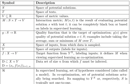
Symbol Description

S Space of potential solutions.

T Space of tests.

V ⊆_R Space of metric values.

M :S×T →V Interaction metric; M(s, t) is the result of evaluating potential solution swith test t; it can be completely black box or based on labels in supervised learning.

g:S →R Quality function that is the target of optimization; g(s) gives

quality of potential solution s∈S; examples include taking the average, sum or minimum of M overT.

X Space of inputs, from which data is sampled.

Y Space of outputs (labels for inputs).

f :X→Y Target function from YX, labeling inputs; it defines M when viewing supervised learning as co-optimization.

D⊂X×Y Data set of size nfrom which f must be inferred. D = (xi, f(xi))i=1..n

H In supervised learning, set of hypotheses considered (also called a model). In co-optimization, set of potential solutions actu-ally being searched. Its mapping to YX or, respectively, S is typically not one-to-one.

Table 1: Notation summary for Section 2.1 (Problems) and Section 2.2 (Algorithms).

of labels, a strict subset X0 = (xi)i=1..n of X and access tof in black-box fashion with the

restriction that we can only queryf forxi ∈X0.

If mapping this to co-optimization, the restriction on access tof means in turn that we can only get the value of M for pairshs, xji for thosexj ∈X0 for which we have obtained

a label. However, while in generic co-optimization one metric evaluation is the basic unit of cost, in active learning if we perform multiple M(s, xj) evaluations with differentsbut

the same xj we incur the cost of obtaining the label f(xj) only once overall and the costs

fors(xj) and δ(s(xj), f(xj)) multiple times, once for eachs.

This is true for two additional flavours of active learning. One further variation of the above problem consists of the case when we are not provided with a setX0⊂X, but with a stream of elements fromX: each element is available only for a limited time, during which the algorithm can ask for a label for that element, thus it must decide quickly whether or not to do so—and we cannot ask for all labels. This setup is of interest for domains such as part-of-speech tagging (Dagan and Engelson, 1995).

can be generated de-novo. Consequently, if we model this as co-optimization, we have no restrictions in terms of which pairshs, xiwe can compute M for. Thus, this problem is the most similar to the co-optimization problems of resilient piping design and sorting network design. The difference is that for those problems it wasM directly that was given in black-box fashion, whereas for the de-novo active learning problem we have that M is defined through f and it is f that we have black-box access to. The impact of this difference will be discussed in Section 3.

For all active learning problems there may be a budget constraining how many labels the algorithm can obtain.

2.2 Algorithms

We now turn to discussing the various types of algorithms that have historically been used to approach supervised learning and co-optimization problems. Even state-of-the art algorithms tend to fall under these broad types or employ as components the core approaches described here and hybrids thereof; when they don’t, this framework should make it easy to express how they differ. Our categorization is mainly driven by the way algorithms make use of the information available to them. Sections 2.2.1 and 2.2.2 will read familiar to the machine learning researcher; we review some basic notions so that: 1) whenever possible, we can directly describe them using co-optimization terminology; and 2) we can refer back and contrast with them the co-optimization-specific notions we introduce later in Section 2.2.3 and thus build towards the vocabulary mapping in Table 3.

2.2.1 Supervised Learning Algorithms

Recall from the formalization of supervised learning in Section 2.1.2 that we are looking for an element s ∈ S that minimizes g(s) = P

t∈TM(s, t) =

P

t∈T(1−δ(s(t), f(t))), but we

only have access to the value off(t) fort∈(xi)i=1..n from the data D. Thus, a first issue

to be addressed is that we cannot actually compute g(s) for any s. Supervised learning algorithms deal with this by working with restrictions of the sum inside g to subsets of the data. State-of-the-art methods employ meta-approaches such as regularization or cross-validation (discussed at the end of this section), but at their core they incorporate and expand upon the following procedure. Data is randomly partitioned into a training set and a test set. Ans∈S is identified that minimizes gtr_{, the variant ofgobtained by summing}

M(s, t) only over the t in the training set, also called in-sample error or training error. It is hoped that gtr(s) will correlate with the actual value of g(s), though of course the former is an optimistically-biased estimator of the latter. For that reason, for the best s only, an unbiased estimator is computed by summing M(s, t) only over the t in the test set. Overfitting or over-training is said to have occurred if an s was chosen that had low training error, but high test set error. The term generalization error is used to refer either to the actual value ofg(s) or to the out-of-sample error defined as the sum ofM(s, t) only over thet∈T \(xi)i=1..n (the symbol ‘\’ stands for set difference).

that implements f or a good approximation of f. The elements of H are referred to as hypotheses. For instance, H could be the set of neural networks of a particular size and shape, or the set of decision trees of a certain depth, etc. Such a setH is typically called a model.5 There may be multiple elements of H that implement the same function from X

toY and there may be functions from X toY that no element of Himplements (i.e., the mapping from H toYX is not one-to-one). The choice of H (and an algorithm to search it) has a strong bearing on the expected generalization error and carries with it a so-called bias-variance tradeoff (Geman et al., 1992), where bias and variance represent two different sources of said error that are difficult to minimize simultaneously. Bias is the average, over possible data sets, of the distance between the target function and the best hypothesis found by the algorithm for that data set. The variance measures how much this best hypothesis varies with the data set. Larger, more complex setsH tend to have lower bias but higher variance and be prone to high generalization error via overfitting. Smaller and simpler sets

H tend to have lower variance but be prone to high generalization error due to high bias (underfitting).

For many supervised learning approaches, the choice ofHrequires that the data is either directly given as or can be transformed into tabular form, i.e., the set X can be written as

Xf=X₁f×X₂f×...×X_kf where the setsX_ifare numeric, ordinal or categorical in nature (the superscript ‘f’ stands for ‘feature’). These sets represent so-called variables or features or (in statistics) covariates. In certain domains the elements ofXin fact have richer structure, which cannot be represented in tabular form. When mapping such anX into anXf there will inevitably be information loss; additionally, the choice of mapping could have an impact on the difficulty of the problem.

At the core of even sophisticated machine learning methods there are two main ways in which the structure ofHhelps locate an element ofHthat minimizesgtr and they differ in the way they make use of the training data: constructive versus exploratory.6

Constructive approaches rely on a mapping of X toXf and defineH in such a way that the training data can be used to directly construct asingle elements∈ H with a good

gtr-value (low training error). From a co-optimization standpoint, this constructive process used during training does not involve any M(s, t) evaluations. For instance, for decision trees (Rokach and Maimon, 2014) this is done by repeatedly partitioning the examples based on one feature X_if at a time, by using the relationship between the feature’s values for the training data points and the respective labels of those data points; a new node is added to the tree with each partition until a maximum depth is reached. For support vector machines (SVMs, Cristianini and Shawe-Taylor, 2000), H is a set of polynomials which, along with some constraints, makes the problem of minimizing training error into a quadratic programming problem.

Exploratory approaches work by computing the training error gtr for multiple ele-ments of Hin order to find one with a good value. In co-optimization lingo, they perform a series of M(s, t) evaluations for various s∈ Hand various tin the training set portion of (xi)i=1..n in order to decide whichsto pick. This search process can be strongly or loosely

guided.

5. In some works, the word ‘model’ is used to mean a single hypothesis. To avoid confusion, in this paper

‘model’ only refers to a set of hypothesesH.

One way to provide strong guidance to the search is to map X to Xf and define the spaceHso that the errorgtrhas a closed form with easily computable derivative that allows gradient descent techniques to be used for minimization. Neural networks are an example of this (Rumelhart et al., 1986): the X_if are mapped to the input nodes of the network,

H is the set of all possible weight combinations for the edges and the error function is linear in these weights. Forward propagation constitutes performing one M-evaluation.7 Back-propagation of the error to update the weights via gradient descent generates a new network s0 ∈ H. Using a single example for each back-propagation step generates a series of evaluations of the type M(s1, t1),M(s2, t2),M(s3, t3), . . .. Using multiple examples and aggregating the error before propagating it back leads to a series of evaluations of the type

M(s1, t11),M(s1, t21), . . . ,M(s1, t1i),M(s2, t21),M(s2, t22), . . . ,M(s2, t2j), M(s3, t31), . . .. In

ei-ther case, the swith best gtr-value (often last in the series) is output. Choosing the order in which to use the examples is typically done stochastically and orderings resulting from different random seeds lead to different exploratory paths through H.

An example of a loosely-guided exploratory approach is the application of genetic pro-gramming (Koza et al., 2006) to supervised learning. Genetic propro-gramming is a set of techniques from the field of evolutionary computation (De Jong, 2006) that draw inspira-tion from the principle of evoluinspira-tion by natural selecinspira-tion to search for computer programs achieving some task. Programs can take various shapes, such as rule-sets in the field of learning classifier systems (Lanzi et al., 2003), expression trees in symbolic regression (Icke and Bongard, 2013), even neural networks with variable structure in neuro-evolution (Flore-ano et al., 2008), etc. The setX, representing inputs to the programs, need not necessarily take tabularXfform and the spaceHof programs is not constrained to lead to a closed-form error function. Instead, H is endowed with a topology such that neighboring points (pro-grams) inHhave close error values. This topology is induced by so-called genetic operators that generate new programs in H from previous programs, in a manner inspired by how mutation and crossover work on DNA. A programs∈ His evaluated by computingM(s, t) for some (usually all)tfrom the training-set portion of (xi)i=1..nand aggregating these

mea-surements into one value, often referred to as fitness. Programs with good fitness (low error) are selected and operators are applied to them to produce a population of new programs; the process then repeats for multiple iterations called generations. These techniques are slower at climbing any given local optima than pure-gradient methods—since they essen-tially have to indirectly estimate the gradient by performingM(s, t) evaluations—but better at avoiding getting stuck in one. Note also that they are general optimization techniques applicable to other tasks besides supervised learning and therefore not tuned to it.

Meta-approaches. Both exploratory and constructive approaches need to be con-cerned about over-/under-fitting. One heuristic is to try out setsHof different complexities: for example, put a hard constraint on the degree of the polynomials or the depth of the trees considered, then investigate what happens when varying the value of the constraint. Another heuristic is to use “soft” constraints, i.e., allow an all-encompassingH, but include in the training error gtr a penalty term for the complexity of individual hypotheses in that

H; examples include: allowing trees of high maximum depth, but including a penalty term that grows with the depth; or allowing polynomials of high degree, but including a penalty

7. Feeding exampletthrough networkscomputess(t) and determining disagreement between the network’s

term that is low when most weights are close to 0 and high otherwise. This latter heuristic is generally referred to as regularization; in genetic programming, penalizing tree depth is called parsimony pressure. Different levels must be tried out for the relative contribution of the penalty term versus the main error term.

In the above, the expression ‘try out’ refers to the fact that the overall algorithm applies multiple basic methods (either exploratory or constructive), or applies a parameterized ba-sic method multiple times with different parameter values, then selects one of the variants for producing the final output—a process known as model selection. To perform the selec-tion, (semi)unbiased empirical estimates are computed for the output of each variant by performing additional M(s, t) evaluations with tests not used during the training of that variant—a process known as (cross-)validation (Refaeilzadeh et al., 2009; Geisser, 1975; Stone, 1974). Thus, during this process, what was originally designated as a training set gets further split (possibly multiple times for cross-validation) into an actual training set and a validation set. The term holdout set has also been used in the literature, but with inconsistent meaning, referring sometimes to a validation set and sometimes to a true test set. The test set is still to be used only once to get an unbiased estimate for the quality of the final output. Such uses of estimates for output selection and performance evaluation are relevant for co-optimization algorithms as well, as discussed in sections 2.2.3 and 2.3.2.

2.2.2 Active Learning Algorithms

Typical approaches to active learning treat the problem as an extension of supervised learn-ing. As such, they use a query strategy to decide for which pointsx∈X to obtain a label, then apply one of the supervised learning methods described above on the labeled data accumulated so far, then re-iterate these two steps. Some query strategies are generic and could be used with any supervised learning approach, whereas others are specific to the supervised learning algorithm used (Settles, 2012). Whether the core supervised learning approach is constructive or exploratory,the query strategy of active learning algorithms can

be thought of as exploring the set X. The resemblance of active learning to co-optimization

suggests there may be approaches that are more direct than the standard iterative one. We will revisit this at the end of Section 3.

2.2.3 Co-optimization Algorithms

Because in co-optimization it is the metricM that is given in black-box fashion (as opposed to anf that further definesM), it is not obvious if or how one could find a good element of S through a constructive approach. Therefore, co-optimization algorithms (Service and Tauritz, 2008a) are exploratory by necessity and involve adaptations of stochastic search and optimization heuristics (Luke, 2013) like simulated annealing (SA), hill-climbing (HC) and evolutionary algorithms (EAs)—the genetic programming described in Section 2.2.1 being an example of the latter.

way the space S is represented in the computer often means that what’s actually being explored by the algorithm is a set other thanS and whose mapping toS is not one-to-one. To limit notation, we’ll denote this set by the same symbolH. In the field of evolutionary computation (De Jong, 2006), the choice of H is called a representation and the mapping from Hto S is called the genotype-to-phenotype mapping. One still needs to consider the tradeoff between the ability of H to represent many/all the elements of S and the ease of searching H (which may decrease as the size of H increases). This can be considered a counterpart concept to supervised learning’s bias-variance tradeoff.

As in supervised learning, an important issue is the fact that we might not be able to compute the actual value of the quality functiong that we are to optimize, because g(s) is defined as the sum ofM(s, t) forall t∈T andT is very large and/or M is very expensive. In contrast to supervised learning, there are no restrictions as to which elementst∈Twe can use inM(s, t) evaluations. Consequently,co-optimization algorithms explore not just the

spaceS but also the spaceT, as well as the cross-product of the two. Thus, a co-optimization

algorithm can be formalized as having two components: 1) the exploration mechanism,8 deciding which interaction between a potential solution s∈ S and a test t∈ T should be evaluated next via the metricM, given the sequence of interactions previously evaluated and their M-values, also referred to as the history9; and 2) the output mechanism,10 deciding, based on such a history, which potential solutionsto output. This formalism can be used to describe exploratory approaches to supervised learning as well; and most meta approaches perform some kind of output selection even when incorporating constructive components.

Exploration mechanisms. A basic but sometimes successful approach is to use any of the previously-mentioned stochastic search heuristics for exploring S, by evaluating any considered s∈S with a random sample of tests t∈T and using as fitness an aggregation of the resulting M-values, a placeholder for the true quality ofs. This sample may contain a portion that is fixed throughout the entire algorithm, a portion that is regenerated for each iteration and a portion that is regenerated for each s.

Another popular approach is to apply the evolutionary metaphor to both spaces. The resultingcoevolutionaryalgorithms (Popovici et al., 2010) maintain a population of potential solutions s ∈ S and a population of tests t ∈ T. Elements in the former population are paired with elements in the latter and the resulting interactions are evaluated via the metric

M. Various interaction methods can be used to determine who is paired (interacts) with whom (Popovici, 2006). For the maxiavg/maxisum solution concepts, fitness is typically assigned to each elementsin the S-population by averagingM(s, t) for all the interactions that particularswas involved in; such fitness represents a subjective quality, internal to the algorithm. Much research has gone into how to assign fitness to the elements ofT, leading to two main paradigms: 1) if high values ofM are good for the elements ofS, then reward tests in T for low values of M (i.e., for being difficult tests)—a paradigm traditionally

8. This has also been called just analgorithm(Wolpert and Macready, 2005; Service and Tauritz, 2008b) or

asearch heuristic (Service and Tauritz, 2008b; Service, 2009a,b; Popovici and De Jong, 2009; Popovici

et al., 2011).

9. This has also been called asample (Wolpert and Macready, 2005) or simply a sequence (Service and

Tauritz, 2008b).

10. This has also been called achampion-selection rule (Wolpert and Macready, 2005), achampion selection

function(Service and Tauritz, 2008b), acandidate selection function(Service and Tauritz, 2008b; Service,

referred to as competitive coevolution (Angeline and Pollack, 1993; Popovici et al., 2010); and 2) reward elements of T for their ability to differentiate between elements ofS, that is for beinginformative tests (Bucci, 2007). In addition to the tests in the current population, archives of hard/informative tests can be kept and used in evaluations (Rosin and Belew, 1997; de Jong, 2005). Co-optimization problems emerged as a formalization of the kinds of problems coevolutionary algorithms were being applied to.

Both approaches (random sampling of tests versus coevolution) typically use the same

number of tests to evaluate all potential solutions considered; these potential solutions are

calledpartially evaluated, as said number of tests is usually much smaller than|T|.

Output mechanisms. A typical approach is greedy, which outputs the partially-evaluated potential solution with the best average ofM-values over the tests it was evaluated with. It is also common to maintain archives of promising potential solutions (as identified by the greedy method) and then do another round of M-evaluation for them, with either freshly sampled or similarly archived tests, and pick the output based on the resulting

em-pirical g-estimates (Panait and Luke, 2002); this is similar to the process of validation for

model selection used in supervised learning. Newer work (Wolpert and Macready, 2005) has introduced optimal output mechanisms whose definition makes use of theoretical (Bayes) estimates of g consisting of aggregations (e.g., averages) over all possible values that yet-unperformed metric evaluations could result in. Interestingly—and unlike greedy—such output mechanisms even consider outputting completely-unevaluated potential solutions, i.e., ones for which the algorithm hasn’t yet performed any M-evaluations, if their Bayes estimates are better. We will discuss these in more detail in sections 2.3.2 and 3.

Estimates of g, whether empirical or theoretical, can also be used to judge the quality of the outputted potential solution. In particular, using freshly sampled tests to obtain an unbiased empirical estimate (Chong et al., 2008) is similar to the way a test set is used in supervised learning; such an estimate represents an objective quality and is external to the algorithm itself. As with over/under-training in supervised learning, this is necessary be-cause a disconnect can occur between internal and external quality measurements (Popovici and De Jong, 2005; de Jong, 2007).

2.3 Cost and Performance

In computer science the terms cost and performance are sometimes used interchangeably, especially when algorithms are acceptable only if they produce correct output and differenti-ating between them is done by measuring their execution speed. In supervised learning and co-optimization the notion of correctness is replaced by as-good-as-possible, thus we have to differentiate between two terms. We use the word ‘performance’ to refer to quantities having to do with the quality of potential solutions outputted by the algorithm. We use the word ‘cost’ to refer to time or money. Performance and cost are typically inter-related, since the performance of an algorithm may vary with the cost expended. We start by for-malizing the various types of cost encountered in co-optimization and supervised learning, and hint at possible tradeoffs between different types. Then we review ways of assessing performance, which may itself incur costs.

2.3.1 Cost

In general, costs can take several high-level forms: 1) computational time, that is the time required by a computer to perform a calculation; it can vary from one hardware to another, but may be expressible in terms of basic operations via the big-O notation of traditional computational complexity—this tends to be more difficult to achieve when the calculation is in fact a complex simulation; 2) real-world time, for instance time required to run a physical or chemical experiment, or time required to get a human to provide a label; and 3) money, for instance to pay for a lab, materials and people.

Algorithms for supervised learning and co-optimization problems can incur these kinds of costs while carrying out various activities. Some are directly driven by the problem spec-ification: obtaining labels for active learning and evaluating M(s, t) for co-optimization; all algorithms attacking these problems will necessarily incur the associated costs. Other cost-incurring activities are dependent on the specific choice of algorithm and include: ex-ploration decisions, construction, output selection. Last but not least, in supervised learning and co-optimization evaluating the performance of any algorithm often incurs additional costs. Table 2 provides an overview in concise form.

Labeling costs are relevant only for active learning and are discussed extensively in Section 2.1.4, so we only re-summarize them on the top of Table 2. The only additional note is that while for all the problem examples in Section 2.1.4 labeling costs were in the form of real-world time or money, they can occasionally be measured in computational time: for instance, trying to find a quick-to-compute approximation for a very-slow-to-compute simulation (Sacks et al., 1989), such as one involving computational fluid dynamics or a weather model.

Metric-evaluation costs are part of the problem specification inco-optimization, as detailed in Section 2.1.1; their type and magnitude can vary, but even when computational and small it is a concern due to the very large sizes of S and T (often combinatorial or exponential) requiring a lot of M-evaluations to find good potential solutions.

Metric-evaluation costs are also relevant in supervised learning. They are a key concern for all exploratory algorithms, since exploration decisions are made based on the outcome of such evaluations. Additionally, incurringM(s, t) evaluation costs may also be necessary for two other algorithmic activities discussed later in this section, namely output selection and performance assessment, which are relevant even for constructive approaches to supervised learning. The cost of evaluating M(s, t) is always computational time and has two compo-nents: 1) cost of computing s(t), that is the computational time required to run examplet

Po ol-b ased Str eam -base d De-n ovo Fre e ( "g ift" fr om some one e lse ) Ho w ma ny … Re str icte d b y pr oble m sp ec ific ati on Re str icte d m ai nly by lab elin g b ud ge t, th en b y p b. sp ec . … an d w hich e xam ple s w e can ge t lab els fo r: U nr es tr icte d Mai n c os t o f in te re st, al l al go rith m s in cu r it Ty pe : u su al ly c om pu tati on al , s om eti m es re al -w or ld ti m e an d/ or m on ey Mag nitu de : v ar ie s w id ely , a co nc ern e ve n if sm al l d ue to ex tr em ely lar ge S an d T Ho w ma ny … … an d w hich in te rac tio ns < s , t >: Re str icte d to t in tr ai nin g d ata U nr es tr icte d … to d ec id e w hic h in te rac tio ns to e val uate n ex t: Alw ay s in cu rre d, as al l ap pr oac he s ar e e xp lo rato ry Mag nitu de : n eg lig ib le co m par ed to m etr ic-ev al uati on co sts fo r tr ad iti on al ap pr oac he s ( EA s, S A, HC s), no t s o f or ne w er on es (C MA -E S, E D As , B ay es -o pti m al ) … to d ec id e w hic h e xam ple s to lab el n ex t: N/ A N/ A Mag nitu de : n eg lig ib le fo r g re ed y m eth od s; m ulti ple o f m etr ic-ev al uati on co sts w he n u sin g e m pir ical e sti m ate s; ne glig ib le to p ro hib iti ve fo r th eo re tic al B ay es e sti m ate s Mag nitu de : m ulti ple o f m etr ic-ev al uati on co sts w he n us in g e m pir ical e sti m ate s; n eg lig ib le to p ro hib iti ve fo r th eo re tic al B ay es e sti m ate s Test-b ased Co -o pti mi zati on N ot ap plic ab le (N /A ), th ere ar e n o lab els Labe ling c osts Supe rvise d Le ar ning Pay fo r lab el Ty pe : u su al ly m on ey o r ti m e, o cc as io nal ly c om pu tati on al . Mag nitu de : v ar ie s w id ely ac ro ss do m ai ns Ac tiv e Pa ssi ve Labe l availability M( s , t ) av ailability Me tric -e va lu ati on (M( s , t )) costs May al so b e in cu rre d as p ar t o f o up ut-se le cti on an d p erf or m an ce -as se sm en t Re str icte d b y lab elin g b ud ge t Re str icte d Re str icte d to t th at w e h av e c ho os en to o btai n a lab el f or (se e lab el av ai lab ility ) Re str icte d b y m etr ic-ev al uati on b ud ge t Ty pe : al w ay s c om pu tati on al , tw o c om po ne nts s(t) an d δ(s (t) , f( t) ) ; ex cl us ive of co st of ob tai nin g lab el f(t) In cu rre d d ur in g tr ai nin g b y e xp lo rato ry al go rith m s In cu rre d d ur in g te sti ng an d v al id ati on b y al l al go rith m s Co st of s(t) al w ay s in cu rre d in th e r eal w or ld b y d ep lo ye d s olu tio n Mag nitu de : s(t) var ie s w ith h yp oth es is s ize , δ w ith lab el s ize N/ A Co nst ru ct io n co st s

Type: allways computational

Ou tp ut -sel ect io n co st s

Type: usually computational, unless we collect new data or perform new experiments

For active learning, note that the cost of obtaining the label f(t) is not included in the cost of M(s, t), because a label can be used for multiple computations of M(s, t) for the sametbut different s.

Exploration-decision costs are incurred to decide which problem-specification costs to incur next (e.g., which evaluationsM(s, t) an exploratory approach would perform, or, in the case of active learning, which labels a query strategy would request). They are always computational.

Back-propagation in neural networks for supervised learning is an example of an explo-ration decision incurring a cost: it produces a new network s for which to then evaluate

M(s, t) via forward propagation. The cost of one backward propagation has similar mag-nitude to that of one forward propagation and both vary with the size of the network, as described earlier. If multiple rounds of forward propagation are performed for each back-ward propagation, then, overall, exploration-decision costs are accordingly smaller than metric-evaluation costs.

Evolutionary approaches, whether used for supervised learning orco-optimization, usu-ally incur exploration-decision costs while performing selection and breeding to produce a new generation of potential solutions, which will then be involved in M(s, t) evaluations. Similarly, simulated annealing and hill-climbers incur exploration costs when generating and sampling from a local neighborhood. Historically, these costs have been considered much lower than M(s, t) costs. But newer stochastic black-box optimization heuristics tend to have non-negligible exploration costs, such as: quadratic matrix computations for covariance-matrix adaptation evolutionary strategies (CMA-ES, Hansen and Ostermeier, 2001), estimating distributions for estimation of distribution algorithms (EDAs, Larranaga and Lozano, 2002), recursive optimization for optimal exploration mechanisms (Popovici and Winston, 2015; Popovici, 2017).

In active learning, exploration-decision costs are also incurred via the query strategy

used to decide the nextx∈X for which to obtain a label. Such costs vary widely with the strategy (Settles, 2012) and have to be weighted against the costs of obtaining labels, since reducing the latter is the main goal of sophisticated query strategies .

Construction costs, as the name suggests, are incurred by constructive approaches to supervised learning, whether passive or active; examples include the construction of a decision tree and solving quadratic programming equations for support vector machines. They are computational costs, usually measured in basic operations and expressed via big-O complexity as a function of properties of the problem, such as size of data. They are of particular concern for the increasingly more common “big data”, as well as in active learning, where these costs are incurred multiple times if full retraining is necessary each time new labels are obtained.

In co-optimization, simple output selection methods just side-step the issue, by using the greedy heuristic of outputting the potential solution with the best average over only the tests seen so far, a highly-biased empirical estimate of g. Keeping track of this potential solution is trivial, so output selection costs have historically been considered negligible compared to metric-evaluation costs. As described in Section 2.2.3, there are also approaches that acknowledge the issue. Some compute new empirical estimates of g for a handful of potential solutions identified via the greedy method, then use these estimates (which could be unbiased or at least less biased) to select which one to output; this requires performing additional M(s, t) evaluations and incurring the respective metric-evaluation costs. Others use theoretical g-estimates whose computation does not involve performing additional metric evaluations, but rather aggregating (e.g., averaging) over all possible values that such evaluations could result in. These aggregates can be computationally-prohibitive; but output selection only relies on comparisons between them, the outcome of which can sometimes be determined without actually computing the aggregates themselves (Popovici and De Jong, 2009; Popovici et al., 2011; Popovici, 2017), in which case the costs are minimal.

Unless we collect new data or perform new experiments for the purpose of additional

M(s, t) evaluations, output selection costs are only computational. This is the case for su-pervised learning as well. Here too, output selection costs can be negligible if the algorithm simply outputs the outcome of the training process for a particular method, for example, the decision tree constructed, or the final set of weights for a neural network (which is often the greedy best-so-far, given the gradient-based nature of exploration via back-propagation). More commonly though, a model is selected first via (cross-)validation, as described in Section 2.2.1. To compute the empirical estimates involved in validation,M(s, t) costs are incurred by performing additional metric evaluations for the outputs of the models to be selected amongst.

2.3.2 Performance

By performance of an algorithm we mean the quality of the algorithm’s outputted potential solutions with respect to the problem solving goal. But because in supervised learning and often in co-optimization as well exact quality is not actually computable, assessing algorithmic performance is an uncertainty-laced, more difficult task in these fields compared to traditional function optimization.

Perhaps the simplest performance question one can answer—and one that is quite im-portant to answer in practice—is: on the problem instance at hand, what is the quality of the potential solution that constitutes our algorithm’s final choice as the solution to be deployed in the real-world?

This is a quality-estimation question, so it can be answered the same way as when part of the output selection process (see previous section). But subtle care must be taken. Computing unbiased empirical estimates (by performing additionalM(s, t) evaluations and incurring the associated costs) must be done with fresh tests in co-optimization (Chong et al., 2008) or, in supervised learning, with labeled data points (a test set) not used for any other purpose.11 Moreover, the resulting estimate should not be used for any further

tweaking of the chosen potential solution, or else it ceases to be an unbiased estimate; in other words, a true test set is always single-use—but see the work of Dwork et al. (2015) for a novel technique where the bias resulting from reuse is small and quantifiable as a function of the amount of reuse.

We may also wish to know how performance of an algorithm varies as a function of given resources/cost expended, so we can determine how we may be able to boost performance. Ideally, such characterizations would take into accountall costslisted in the previous section. In reality, different approaches have focused on different aspects of the performance-cost dependence.

In passive supervised learning, the main concern is with performance as a function of resources, in the form of size of available data. However, the cost of acquiring data is not counted as a cost incurred by the learning algorithm. Indirectly, this dependency on data size does describe a relationship between performance and algorithmic cost, be-cause making use of more data takes more time, whether it is done in constructive or exploratory fashion. Because of this, a whole subfield of supervised learning concerns itself with instance selection, that is determining a subset of the labeled examples that is small, yet using it would result in similar output quality as using the whole set (Reinartz, 2002). In co-optimization, the main concern is with performance as a function of metric-evaluation costs. In active learning, the main concern is with performance as a function of labeling costs. Unlike passive supervised learning, the latter two fields do concern themselves with the dependency of performance on the cost of acquiring data, whether the data consists of values ofM or values of f.

Algorithms often have one or more parameters whose values must be set. Thus an-other important issue is how performance varies with changes in parameters. In supervised learning, a common example of this comes from binary classification in the form of receiver operating characteristic (ROC) curves (Spackman, 1989) which plot how the error for one class changes as a function of the error for the other class while varying the value of the algorithm parameter investigated.

Being able to compare the performance obtained for two different values of one parameter of an algorithm is akin to being able to compare two different algorithms. While empirical quality estimates allow us to do that and to determine if one one algorithm is better than another for the one problem instance at hand, the question that immediately arises is whether some algorithms are better than others in a general sense (i.e., across all, or a large class of problem instances). This is important because designing or tuning a new algorithm for each problem instance is a time-consuming manual activity that might not be feasible in practice. For instance, imagine a factory that must schedule jobs on a set of machines susceptible to various breakdowns (Jensen, 2001) and must produce a new schedule every day for the jobs of that day. One cannot re-tune with such high frequency.

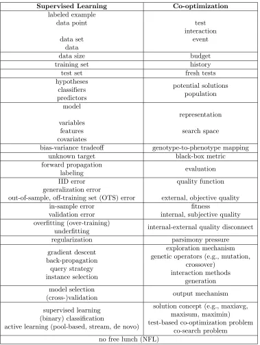
Supervised Learning Co-optimization

labeled example data point

data set data

test interaction

event

data size budget

training set history

test set fresh tests

hypotheses classifiers predictors

potential solutions population

model

variables features covariates

representation

search space

bias-variance tradeoff genotype-to-phenotype mapping

unknown target black-box metric

forward propagation

labeling evaluation

IID error generalization error

out-of-sample, off-training set (OTS) error

quality function

external, objective quality in-sample error

validation error

fitness

internal, subjective quality overfitting (over-training)

underfitting internal-external quality disconnect

regularization parsimony pressure

gradient descent back-propagation

query strategy instance selection

exploration mechanism genetic operators (e.g., mutation,

crossover) interaction methods

generation model selection

(cross-)validation output mechanism

supervised learning (binary) classification

active learning (pool-based, stream, de novo)

solution concept (e.g., maxiavg, maxisum, maximin) test-based co-optimization problem

co-search problem no free lunch (NFL)

rather than on the overall errorg(IID error, where IID stands for independently identically distributed). For the OTS notion, he showed that there is no free lunch (NFL), meaning that for any given data set: 1) if all hypotheses consistent with that data set are equally likely (i.e., uniformly distributed), then all algorithms have the exact same aggregated per-formance; and 2) for any two algorithms, there are as many distributions over hypotheses for which one algorithm is aggregately-better than the other for that data set, as there are distributions where the opposite relation between algorithms holds. If by ‘better’ we mean better actual g value (i.e., over all tests in T), then there is free lunch, but of a rather un-satisfying type: the only aggregate-performance differences between algorithms come from their in-sample error. And while overall error is non-increasing as a function of the data set sizen, out-of-sample error can actually increase with n (Wolpert, 1992). All of this holds regardless of the amount of computation expended by the algorithms.

Wolpert and Macready (2005) adapted and applied this approach to co-optimization. Since in co-optimization there is no given data set, the meaning of ‘better’must rely on the actual value ofg over all tests inT and the “fair ground” on which we compare algorithms is not a data set but the budget ofM(s, t) evaluations they are allowed to perform. Under this setup, there is free lunch (i.e., some algorithms are aggregately-better than others)even if all metricsM are equally likely.12

Active learning has not been studied to a similar extent from a free lunch perspective. Cursory treatment by Wolpert (1996) claims negative implications of no free lunch theorems apply just as they do for passive supervised learning. The details of this are unclear though, as there are several different NFL theorems for passive supervised learning and they are conditioned on a given data set (or its size) and are generally concerned with error outside this data set, whereas in active learning there is no data set given upfront, generating data is a key part of the algorithms. The claim is also intriguing given active learning’s similarities with co-optimization and the existence of free lunch in that field. Investigating this issue is subject for future work and the treatment in Section 3 should provide a base towards that: it uses the common ground built in Section 2 to get a deeper understanding of the commonalities and differences between the two fields from a free lunch perspective.

3. Free Lunch Study

Having laid out the various concerns and approaches to measuring performance and cost, we now use them to present a proof-of-concept method transfer from co-optimization to supervised learning. Specifically, we focus on the free lunch view of performance versus cost, where quality is measured by means of theoretical Bayes estimates and metric-evaluation costs are constrained by a budget. We show how optimal exploratory algorithms can be designed within this framework, but also emphasize how they might incur significant costs in some of the other categories listed in Section 2.3.1, such as exploration-decision costs and output-selection costs, thus arguing for the need of a more encompassing view on costs to be developed.

We structure the presentation in 3 incremental steps with respect to metric-evaluation costs: in Section 3.1 we describe the small-scale case of only one or twoM-evaluations in to-tal at most one of which is remaining in the budget; in Section 3.2 we progress to histories of arbitrarily-many already-evaluated interactions, but still at most one remaining to be evalu-ated; finally, in Section 3.3 we discuss the most general case of arbitrarily-large spent budgets and arbitrarily-large remaining budgets. In each section we first review the co-optimization perspective and results pertaining to free lunch and optimality, then derive and contrast their counterparts for supervised learning. We focus specifically on binary classification, but many of the ideas presented would apply in a multi-class situation. Throughout, we differentiate between the nature of free lunches for output mechanisms versus exploration mechanisms. We keep the presentation as informal as possible and support it with small but concrete examples; precise mathematical definitions of all concepts involved and proofs of the results can be found in the accompanying Online Appendix A.

3.1 Small Overall Budget

In this section we look at a spent budget of 0 or 1 evaluations and a remaining budget of 1.

3.1.1 Co-optimization

Consider a domain with S = {a, b, c}, T = {t1, t2}, V = {0,1} and M : S ×T → V, meaning there are 3 potential solutions, 2 tests and binary outcomes for interactions between solutions and tests. To ease comparison with supervised learning, suppose the values in V

represent some kind of penalty, such that lower values are better and we’re trying to find the potential solution minimizing the sum of M over the tests (i.e., a minisum solution concept rather than maxisum). The total number of interactions is |S| · |T|= 3·2 = 6 and therefore the total number of possible metrics M for this domain is |V||S|·|T| _{= 2}6 _{= 64.} These are shown in columns 1–7 of Table 4, one per row, numbered from 0 to 63.

Output mechanisms concern themselves with which potential solution to output given the history of interactions evaluated so far and their M-values; this history reflects the budget spent so far; the remaining budget is not a concern. If the current history is an empty sequence H = [] (i.e., we haven’t yet performed any evaluations, spent budget is 0) and we have no other information, then all 64 metrics are possible and, we assume, equally likely (more on this in Section 3.4). Columns 8–10 in the table show, for each metric, the actual value ofg (i.e., the sum ofM over all tests) for each of the 3 potential solutions. At the bottom, the expected value of g, averaged over all metrics, shows that in the absence of any data or information all 3 potential solutions are equally promising, with an expected

g-value of 1. Due to the equal likelihood of all metrics, this can also be thought of as follows: the expected M-value for a potential solution on a test it hasn’t yet seen is the average of the values inV, which is 0.5; summing that over two tests gives 2·0.5 = 1.

Consider now the situation where an algorithm has evaluated the interactionha, t1i and observed value M(a, t1) = 1, so now the history is H = [hha, t1i,1i] (spent budget is 1). What should the algorithm output as the most promising potential solution? As we can see from the columns 11–13 in Table 4, metrics from 0 to 31 are no longer possible, since they have M(a, t1) = 0. Averaging g only over the remaining metrics (which we say are