Numerical method for the 2D simulation of the respiration.

(1)

M. Ismail, B. Maury & J.-F. Gerbeau, Editors

NUMERICAL METHOD FOR THE

2D SIMULATION OF THE RESPIRATION.

∗

A. Devys

1,2

, C. Grandmont

3

, B. Grec

4

, B. Maury

5

and D.Yakoubi

3

Abstract. In this article we are interested in the simulation of the air flow in the bronchial tree. The model we use has already been described in [2] and is based on a three part description of the respiratory tract. This model leads, after time discretization, to a Stokes system with non standard dissipative boundary conditions that cannot be easily and directly implemented in most FEM software, in particular inFreeFEM++ _{[11]. The objective is here to provide a new numerical method that could}

be implemented in any softwares. After describing the method, we illustrate it by two-dimensional simulations.

Résumé. Dans cet article nous nous intéressons à la simulation du flux d’air dans l’arbre bronchique. Le modèle que nous utilisons a déjà été décrit dans [2] et consiste en une description selon trois parties de l’arbre respiratoire. Ce modèle nous conduit, après discrétisation en temps, à un problème de Stokes avec des conditions au bord dissipatives non usuelles qui ne peuvent être implémentées facilement et directement dans la plupart des logiciels utilisant la méthode des éléments finis, en particulier

FreeFEM++ _{[11]. L’objectif ici, est d’apporter une méthode de résolution implémentable dans tout}

logiciel EFM. Apr`es une description de la m´ethode, nous l’illustrerons par des simulations 2D.

Introduction

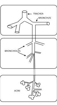
Breathing involves gas transport through the respiratory tract with its visible ends, nose and mouth. The bronchial tree which ends in the alveoli is embedded in a viscoelastic tissue, the whole being enclosed below by the diaphragm and laterally by the chest wall. The air movement is achieved by the displacement of the diaphragm and of the connective tissue framework of the lung (in the sequel we will talk about the parenchyma). The respiratory tract has a quite complex geometry: it is a tree composed by 23 generations which should be implemented (see Fig. 1). At the time being, the distal airways from generation 9 cannot be visualized/segmented by common medical imaging technologies for instance. Consequently it is necessary to elaborate some simple

∗_{This work was partially funded by the ANR-08-JCJC-013-01 project headed by C. Grandmont.} 1

UST Lille, Lab. P. Painlev´e, Cit´e Scientifique, F-59655 Villeneuve d’Ascq Cedex, France; e-mail:[email protected]

2

INRIA Lille Nord Europe, SIMPAF Project team, B.P. 70478, F-59658 Villeneuve d’Ascq Cedex, France;

3

INRIA Paris-Rocquencourt, REO Project team, BP 105, F-78153 Le Chesnay Cedex, France; e-mail:[email protected] & [email protected]

4

Universit´e Claude Bernard Lyon 1, Institut C. Jordan, F-69622 Villeurbanne Cedex, France; e-mail:[email protected]

5

Université Paris-Sud, Laboratoire de mathématiques, Bâtiment 425, bureau 130, F-91405 Orsay cedex, France; e-mail:[email protected]

c

EDP Sciences, SMAI 2009

(2)

Figure 1. Decomposition of the respiratory tree in three parts.

but realistic mathematical model, in order to provide a better understanding of the different lung pathologies and to supply to the limit of medical imaging.

The model of the respiratory tract we consider has already been described by C. Grandmont, Y. Maday and B. Maury in [9] and previously in [2], [10], [18] where similar models are presented. Note that the same kind of multiscale models arises also for blood flow simulations (see for instance [15], [16] and [7]). The idea is to decompose the respiratory tract in three parts:

• the upper part (up to the 7th–9th generation), where the incompressible Navier–Stokes equations hold to describe the fluid;

• the distal part (from the 8th–10th to the 17th generation), where one can assume that the Poiseuille law is satisfied in each bronchiole;

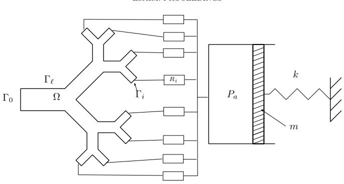
• the acini, where the oxygen diffusion takes place and which are embedded in an elastic medium, the parenchyma. We will suppose that the pressure is uniform in the acini, equal to Pa (an average alveolar pressure), and that they are embedded in a box representing the parenchyma. The motion of the diaphragm and the parenchyma is described by a simple spring model. Figure 2 illustrates, in a synthetic way, this multiscale decomposition: in the proximal part Ω we assume that the Navier–Stokes equations hold true and that they are coupled with Poiseuille flows which are themselves coupled with a spring motion. This spring describes the motion of the diaphragm muscle that is supposed to move in only one direction.

The inlet of Ω is denoted by Γ0, and the outlets are denoted by Γi, 1≤i≤N. These outlets are coupled with Poiseuille flows, which are characterized by equivalent resistancesRithat depend on geometrical properties (length and diameter of the bronchus of eachi-th subtree). The constantkrepresents the stiffness of the spring (that characterizes the elastic behavior of the parenchyma), andmis the total mass of the lung.

(3)

Γ0 Ω Γℓ

Γi R_i

Pa

k

m

Figure 2. Multiscale model.

those papers, the authors has to deal with defective boundary conditions. To compute properly the solution they think their defective boundary conditions as constraints and get a formulation involving Lagrange multipliers. Numerically this formulation brings some features that are close to ours and to reduce the problem to simple Stokes problems a spliting method is used. In the last part, we present numerical results, and check that our model, for appropriate parameters, could reproduce some aspects of respiration.

1. _{Problem setting}

1.1. The coupled model

In the upper part, denoted by Ω (see Fig. 2), we assume that the Navier–Stokes equations hold:



         

         

ρ∂u

∂t +ρ(u· ∇)u−µ△u+∇p = 0, in Ω,

∇ ·u = 0, in Ω,

u = 0, on Γℓ, µ∇u·n−pn = −Π0n on Γ0,

µ∇u·n−pn = −Πin on Γi i= 1, . . . , N,

(1)

whereuandpare respectively the fluid velocity and the fluid pressure. On the lateral boundary Γℓ, we impose no–slip boundary conditions on the velocity, whereas on the artificial boundary Γi, 0≤i≤N we consider a pressure force exerted on the boundary. The pressure Π0is given equal toP0the atmospheric pressure, whereas the pressures Πi are unknown and depend on the downstream parts.

Each of the distal subtrees should be a dyadic tree in which we assume that the flow is laminar. Thus, by analogy with an electric network (see for instance [3]), we can consider that the flow is characterized by a unique equivalent resistance of the conducting airways (referred to as lumped model) that depends on each resistance of the local branches (see for instance [13]). Thus, each of the subtrees is replaced by a cylindrical domain, where the flow satisfies Poiseuille’s law:

Πi−Pa =Ri

Z

Γi

(4)

Thanks to the relation (2), the boundary conditions at the outlets Γi write

µ∇u·n−pn=−Pan−Ri

Z

Γi u·n

non Γi i= 1, . . . , N. (3)

These are non standard nonlocal boundary conditions that link the fluid stress tensor and its flux that arise also in blood flow modelling (see [7]). Note that they induce dissipation in the system (see [2]). We will call this type of boundary conditions thenatural dissipative boundary conditions. Next, the lung is enclosed in a box and one part of this box is connected to a spring that governs the diaphragm and parenchyma motion. The equation satisfied by the positionxof the diaphragm writes

m¨x=−kx+fext+PaS, (4)

where fext is the force developed by the diaphragm during inspiration and expiration. It will be the driven force of the respiration. In order to couple this simple ODE to the upper part of the model, we have to define fP that stands for the pressure force applied by the flow on the elastic medium. If we denote byS the surface of the moving box (corresponding to the diaphragm surface), we have

fP =PaS, (5)

thus

Pa =m Sx¨+

k Sx−

fext

S . (6)

Moreover, since we assume that the parenchyma is made of an incompressible medium, the flow volume variation at the outlets is equal to the volume variation of the parenchyma box, thus we have

Sx˙ = N

X

i=1

Z

Γi

u·n. (7)

Note that since the flow is incompressible and since u= 0 on Γℓ, then N

X

i=1

Z

Γi

u·n=−

Z

Γ0

u·n. (8)

Thus the coupled problem can be written as follows

                                   ρ∂u

∂t +ρ(u· ∇)u−µ△u+∇p = 0, in (0, T)×Ω,

∇ ·u = 0, in (0, T)×Ω,

u = 0, on (0, T)×Γℓ,

µ∇u·n−pn = −P0n, on (0, T)×Γ0, µ∇u·n−pn = −Pan−Ri

Z

Γi u·n

n, on (0, T)×Γi, i= 1, . . . , N , m¨x+kx = fext+SPa,

Sx˙ = N

X

i=1

Z

Γi

u·n=−

Z

Γ0 u·n.

(5)

This system of equations has to be completed by suitable initial conditions







(u, x,x)˙ |t=0= (u0, x0, x1), with

∇ ·u0= 0, u0= 0 on Γℓ, andSx1=−

Z

Γ0

u0·n. (10)

One particularity of this system is that all the outlets Γi,1≤i≤N are coupled.

By setting p=p−Pa , according to (6) and since the total volume is preserved, i.e Sx˙ =−

Z

Γ0

u·n, the coupled system can be simplified as follows

                                   ρ∂u

∂t +ρ(u· ∇)u−µ△u+∇p = 0, in (0, T)×Ω,

∇ ·u = 0, in (0, T)×Ω,

u = 0, on (0, T)×Γℓ,

µ∇u·n−pn = −P0n−fext

S n− m S2 d dt Z Γ0 u·n

n − k S2 Z t 0 Z Γ0

u·n−Sx0

n, on (0, T)×Γ0,

µ∇u·n−pn = −Ri

Z

Γi u·n

n, on (0, T)×Γi.

(11)

Consequently, the coupled system (9) reduces to the Navier–Stokes equations, with fluid pressure replaced by the difference between fluid pressure and alveolar pressure, and with generalized natural dissipative boundary conditions. Note that the incompressibility assumption is essential here.

Remark 1.1. We have used the relation N

X

i=1

Z

Γi

u·n = −

Z

Γ0

u·nto simplify system (9), to decouple the outlets Γi and obtain (11). Nevertheless all what will be done hereafter could also be done without using this relation.

1.2. Variational formulation

We introduce the following functional space V ={v∈H1_(Ω)d_, _{∇ ·}_v_{= 0,}_v_{= 0 on Γℓ}_}_._{Assuming that all} the unknowns are regular enough, we multiply the Navier–Stokes equations by a test–fieldvwhich vanishes on Γℓ, and the spring equation by−(1/S)R

Γ0v·n. Using

x=x0− 1

S

Z t

0

Z

Γ0 u·n,

(6)

                           ρ Z Ω

∂tu·v+ρ

Z

Ω

(u· ∇)u·v+µ

Z

Ω

∇u:∇v+ N X i=1 Ri Z Γi u·n

Z

Γi v·n

+m S2

Z

Γ0 ∂tu·n

Z

Γ0 v·n

+ k S2 Z t 0 Z Γ0 u·n

Z

Γ0 v·n

−

Z

Ω

p∇ ·v+Pa N

X

i=1

Z

Γi v·n−

Z

Γ0 v·n

!

=−P0

Z

Γ0

v·n−fext

S

Z

Γ0

v·n+ k S2Sx0

Z

Γ0 v·n

, ∀v∈H1(Ω)d withv|Γℓ = 0.

(12)

Next, considering test functionsvthat are divergence free (i.ev∈V), we obtain a second variational formulation of the coupled problem (11)

                     ρ Z Ω

∂tu·v+ρ

Z

Ω

(u· ∇)u·v+µ

Z

Ω

∇u:∇v+ N X i=1 Ri Z Γi u·n

Z

Γi v·n

+m S2

Z

Γ0 ∂tu·n

Z

Γ0 v·n

+ k S2 Z t 0 Z Γ0 u·n

Z

Γ0 v·n

=−P0

Z

Γ0

v·n−fext

S

Z

Γ0

v·n+ k Sx0

Z

Γ0 v·n

, ∀v∈V.

(13)

Note that here, we have expressed all the quantities with the help of the fluid velocity. The velocity of the spring can be simply recovered thanks to the identity Sx˙ =−

Z

Γ0 u·n.

2. _{Numerical method}

In this section we will first present the numerical method on a linear problem obtained by omitting the convection terms. Then we will explain how it can be adapted to the general case.

2.1. The Stokes system

In this section, we are interested in the following linear coupled system:

                                   ρ∂u

∂t −µ△u+∇p = 0, in (0, T)×Ω,

∇ ·u = 0, in (0, T)×Ω,

u = 0, on (0, T)×Γℓ,

µ∇u·n−pn = −P0n−fext

S n− m S2 d dt Z Γ0 u·n

n − k S2 Z t 0 Z Γ0

u·n−Sx0

n, on (0, T)×Γ0,

µ∇u·n−pn = −Ri

Z

Γi u·n

n, on (0, T)×Γi.

(14)

First we start to discretize in time the coupled problem. Letδt >0 be the time step, andtn ₌_nδt, _n_∈_N_.

We denote by un _and _pn _{the approximate solution at time} _tn_{. The time-integral term}

Z tn

0

Z

Γ0

(7)

following

Z tn

0

Z

Γ0 u·n≈

n X j=0 δt Z Γ0 uj·n

. (15)

The time discretization reads as follows

                                         ρu n

δt −µ△u

n₊_∇_pn ₌ _ρun−1

δt , in Ω,

∇ ·un ₌ ₀_, _{in Ω}_,

un ₌ _0, _{on Γℓ}_,

µ∇un_·_n₋_pn_n ₌ ₋



P0+

fn ext S − kx0 S + kδt S2

n−1

X

j=0

Z

Γ0 uj_·_n

− m

S2_δt

Z

Γ0

un−1_·_n



n

−

_m

S2_δt− kδt

S2

Z

Γ0 un_·_n

n, on Γ0,

µ∇un·n−pnn = −Ri

Z

Γi un·n

n, on Γi i= 1, . . . , N.

(16) In the sequel, we use the following notations

Fn₌_P0₊fextn S −

kx0 S +

kδt S2

n−1

X

j=0

Z

Γ0 uj_·_n

− m

S2_δt

Z

Γ0

un−1_·_n ₍₁₇₎

and

Rδt 0 =

m S2_δt−

kδt

S2. (18)

Note thatFn_{is known as soon as the velocities at the previous time steps have been computed. The problem} (16) can then be written as

                             ρu n

δt −µ△u

n₊_∇_pn ₌ _ρun−1

δt , in Ω,

∇ ·un ₌ ₀_, _{in Ω}_,

un ₌ _0, _{on Γℓ}_,

µ∇un_·_n₋_pn_n ₌ ₋_Fn_n₋_Rδt 0

Z

Γ0 un_·_n

n, on Γ0,

µ∇un·n−pnn = −Ri

Z

Γi un·n

n, on Γi i= 1, . . . , N.

(19)

Consequently, after time discretization, we obtain a generalized Stokes problem with natural dissipative bound-ary conditions. These unusual boundbound-ary conditions coming from the resistance and the mass–spring time– discretization modify the standard bilinear forms associated to a Stokes problem with mixed Dirichlet–Neumann boundary conditions. In particular, if we consider a finite element discretization, they would couple all the de-gree of freedom at each outlet and change the finite elements matrix pattern associated to the velocity dede-grees of freedom. Consequently, they cannot be easily and directly implemented in a any FEM solver, for instance in FreeFEM++, without going deeply into the code.

(8)

pre–compute a set of solutions with Neumann boundary conditions on each Γi, and then to define the solution as a linear combination of these solutions and of a correction term. This correction term solves also a Stokes problem with standard boundary conditions, the coefficients of the linear combination being calculated so that the solution satisfies the dissipative boundary conditions.

More precisely, thanks to the linearity of the system at each time step, the solution (un_{, p}n_{) of (19) can be} decomposed under the shape

          

un ₌ _u_˜n₊ N

X

i=0

αniui and

pn ₌ _p_˜n₊ N X i=0 αn ipi, (20)

where (ui)N

i=0 and (pi)Ni=0do not depend on time, unlike ˜un+1and ˜pn+1 that are correction terms calculated at each time step:

• for alli= 0, . . . N, the solution (ui, pi) is calculated in thepre–processing step(21)

                     ρui

δt −µ△ui+∇pi = 0, in Ω,

∇ ·ui = 0, in Ω,

ui = 0, on Γℓ,

µ∇ui·n−pin = 0, on Γj, forj 6=i , µ∇ui·n−pin = −n, on Γi.

(21)

• Then, at each time step, ˜un _{takes in account the unsteady term}

              

ρu˜ n

δt −µ△u˜

n₊_∇_p_˜n ₌ _ρun−1

δt , in Ω,

∇ ·u˜n ₌ ₀_, _{in Ω}_,

˜

un ₌ _0, _{on Γℓ}_,

µ∇u˜n_·_n₋_p_˜n_n ₌ ₀_, _{on Γi} _i_{= 0, . . . , N.}

(22)

• Finally the coefficientsαn

i are chosen such that the boundary conditions on the outlets Γi are satisfied. This implies that theαn

i,i= 0, . . . , N are solution of alinear system. Linear system satisfied by (αn

i)0≤i≤N:

• On Γ0, we have (µ∇un−pn)n=−Fnn−R0δt

Z

Γ0 un·n

n.Using the relation (20), we obtain

(µ∇u˜n₋_p_˜n₎_n₊ N

X

i=0 αn

i (µ∇ui−pi)n=−Fnn−Rδt0

Z

Γ0 ˜ un_·_n

n−Rδt 0 N X i=0 αn i Z Γ0 ui·n

(9)

Thanks to the boundary condition of the problems (21) and (22), we find

αn

0 =Fn+Rδt0

Z

Γ0 ˜ un_·_n

+Rδt 0 N X i=0 αn i Z Γ0 ui·n

. (23)

• On Γj, j6= 0, in the same way, we obtain

αn j =Rj

Z

Γj ˜ un_·_n

! +Rj N X i=0 αn i Z Γj ui·n

!

. (24)

Let us denote bybn_{= (b}n

j)0≤j≤N ∈RN+1 the vector defined by

         bn

0 = Fn+Rδt0

Z

Γ0 ˜ un·n

, and

bn

j = Rj

Z

Γj ˜ un_·_n

!

, forj= 1, . . . , N,

(25)

and byA= (aij)0≤i,j≤N the following matrix

aij = ˜Ri

Z

Γi uj·n

, fori, j= 0, . . . , N, (26)

where ˜R0=Rδt

0 and ˜Ri=Riifi6= 0.

As a consequence, at each time iteration, (αn

i)0≤i≤N is the solution of the linear system

(I−A)·x=bn. (27)

We can prove easily that the matrix (I−A) is invertible, see [6].

Remark 2.1. The method used is based on the linearity of the problem. Nevertheless, it enables us to deal with these non standard boundary conditions by solving only standard problems.

2.2. Extension to Navier–Stokes problem

We are now interested in the initial problem (11),i.ewe add a convection term (u·∇)uin the fluid momentum equation. The previous method can be used only for linear problems, nevertheless it can be adapted. We use the same pre-processing step computing the solutions (ui)N

i=0 of the Stokes problem (14). In order to be able to apply the same technics as for the Stokes problem, we either treat the nonlinear term explicitly or with the characteristic method. The first one requires a small time step, this is why we choose the second one. The discretization of the first line of (19) becomes

ρu˜ n

δt −µ△u˜

n₊_∇_p_˜n ₌ ρ δtu

n−1_◦_Xn−1_, _{in Ω,} ₍₂₈₎

whereun−1_◦_Xn−1₌_un−1_(x₋_un−1_{(x)δt) and}_x_{is the generic point in}_Rd_.

(10)

The projection method of Chorin [4], [5] (see also Temam [19] and Quartapelle [14]) is frequently employed for the numerical solution of the primitive variable Navier–Stokes equations. This method is based on a time-discretization of the equations governing viscous incompressible flows, in which the viscosity and the incom-pressibility of the fluid are treated within two separate steps. This allows to decouple the computation of the fluid pressure from the one of the fluid velocity.

In this paper, we choose to solve the problem by a mixed method. The mixed formulation is obtained by multiplying (28) by (v, q)∈H1_(Ω)d_×_L2_{(Ω), where} _v _{vanish on Γℓ. Thanks to the incompressibility and the} boundary conditions, we obtain



 

 

ρ δt

Z

Ω ˜

un+1·v−µ

Z

Ω

∇u˜n+1:∇v−

Z

Ω

∇ ·v˜pn+1 = ρ δt

Z

Ω

un−1_◦_Xn−1_·_v,

−

Z

Ω

q∇ ·u˜n+1 = 0, ∀q∈L2_(Ω). (29)

3. _{Numerical simulations}

The method described before has been implemented inFreeFEM++_{(see [11]). We used the mini–element for the} space discretization of Navier–Stokes system, see for instance [1]. We have performed numerical calculations in a 2D idealized bronchial tree (until 3rd-generation, see for instance Fig. 7). Note that the geometrical quantities that define this 2D tree are chosen such that the resistance of the 2D tree is equal to the resistance of a realistic 3D tree (see for instance [18]). In order to have this conservation we will also modify the fluid viscosity (see below). To perform our simulations, we will use the following data

• Mesh Size or geometry: we use a triangulation composed of – Nvertices= 9996 vertices,

– Ntriang= 17340 triangles and – Nedges= 2650 edges.

– The tree geometry is included in a box [−0,22939, 0,24739]×[−0,35569,0].

• Physiological data (Fluid and spring parameters): in order to reproduce experimental curves, we have used physiological data taken close to those from [3], [12]

– m= 0.3 kg, the total mass of the lung.

– S= 0.011 m2_{, the surface of the moving boundary box (diaphragm surface).} – E= 3.32×105_N_·_m−5_{, the lung elastance.}

– k0=E·S2_{= 40.172 N}_·_m−1_,_{the stiffness of the spring.}

– Rout= 1.33·105_Pa_·_s_·_m−3_{, the resistance at each outlet Γi, i}_≥_0. – Rin= 1.12×105_Pa_·_s_·_m−3_{, the resistance at the inlet (trachea).}

(11)

and the 2D fluid Reynolds number is also equal to the 3D fluid Reynolds number (see [18]). Consequently

(12)

3.1. The simplest case

We perform calculations in a case when there is no external force. First the resistance at the inlet is equal to Rinand the resistancesRi at the outlets are all taken equal toRout. Moreover, the spring stiffness kis equal to k0. Initially, we suppose that the spring is elongated such thatx(0) = 0.1 m. We plot at Fig. 3, the volume variationsV =Sxand the air flow through boundary Γ0with respect time.

0 0.0002 0.0004 0.0006 0.0008 0.001 0.0012

0 0.5 1 1.5 2 2.5 3 0 0.0002 0.0004 0.0006 0.0008 0.001 0.0012 0.0014 0.0016 0.0018 0.002

0 0.5 1 1.5 2 2.5 3

Figure 3. Volume variationV =Sx(in m3_{) and air flow (in m}3_·_s−1_{) through boundary Γ0} versus time (in s).

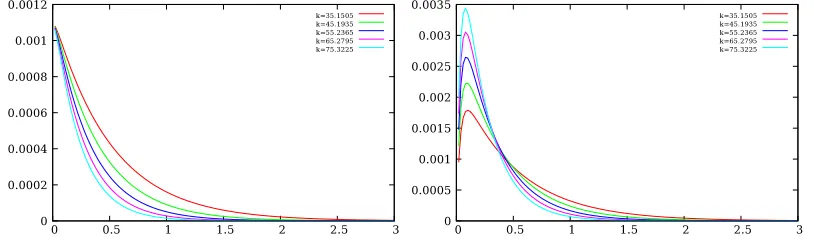
In order to visualize the influence of the stiffness on the system we plot the volume variation V =Sxand the air flow through boundary Γ0versus time for different values ofk, 35< k <75 N·m−1 _{(See Fig. 4).}

Figure 4. Volume variationV =Sx(in m3_{) and air flow (in m}3_·_s−1_{) through boundary Γ0} versus time (in s) for different values ofk.

(13)

Figure 5. Volume variationV =Sx(in m3_{) and air flow (in m}3_·_s−1_{) through boundary Γ0} versus time (in s) for different values ofR,Ri=R0, fori= 1, . . . ,6 andR7=R8=R0×10s_, s=−2,0,3,5.

Comments :

• Whenkis large, the maximal air flux is larger and the spring goes back to its reference position faster (see Fig. 4).

• We note that the change of the values of the resistances for only two outlets (7th and 8th) does not seem to modify significantly the spring relaxation (see Fig. 5).

3.2. Forced respiration

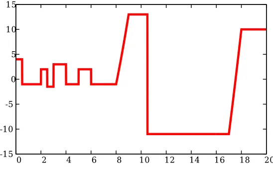
Here we present numerical results obtained in the case of forced maneuvers. These maneuvers are usually performed on patients in order to detect the pathology they suffer. In this case the force fext applied to the spring is given in Fig. 6.

Figure 6. External forcef (in N) versus time (in s).

(14)

lung (and thus onx), see [12]:

k(x) =k+

(fmin/xmin−k)x/xmin, if x≤0

(fmax/xmax−k)x/xmax, if x≥0, (30)

where

• xis, as before, the spring displacement relatively to the equilibrium position. At any time, we have

xmin≤x≤xmax, and we takexmin=−0.25 m andxmax= 0.2 m,

• k0 is, as before, a spring constant, which measures the stiffness related to stretching forces so that the lung comes back to rest spontaneously,

• the external forcefext is a piecewise constant force, with

fmin≤fext≤fmax , fmin=−11 N andfmax= 13 N (See Fig. 6),

and

Ri(x) = Ri 1 +θSx/V0

B

, i= 1, . . . , N, (31)

where

• Riis the airways resistance of the ith subtree at rest, which measures the resistive forces in the bronchial subtree.

• The parameter θdescribes the distribution of the air volumeSxinto the bronchi and the alveoli. The total variation of volumeδV =Sxis the sum ofδVA (for the alveoli) andδVB (for the bronchi) with

δVA= (1−θ)Sx, δVB =θSx.

In what follows, we denote by V0

A (resp. VB0) the air volume in the alveoli (resp. in the bronchi) at rest. See again [18] for more details on this model.

The distribution parameter default value is around 0.4 for a human lungs. When it is lower it may indicate an important smooth muscle activity, in fact a smaller value shows a smaller bronchial tree volume variation, that is to say an important smooth muscle activity.

3.3. A reference case: non pathological data

(15)

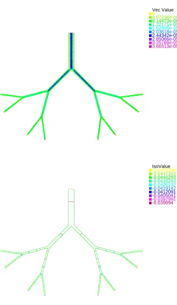
Vec Value

0

4.07236e-06 8.14473e-06 1.22171e-05 1.62895e-05

2.03618e-05

2.44342e-05

2.85066e-05

3.25789e-05 3.66513e-05

IsoValue

-0.0454394 -0.0447343 -0.0440293 -0.0433243 -0.0426192

-0.0419142

-0.0412091

-0.0405041

-0.0397991

-0.039094

(16)

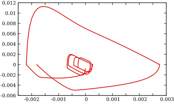
Figure 8. Volume variation (in m3_{) and air flow (in m}3_·_s−1_{) through boundary Γ0} _versus time in forced regime with the physiological data corresponding to a normal patient.

Figure 9. Flow (in m3_·_s−1_{) – Volume (in m}3_{) diagram.}

3.4. Study of sensitivity

(17)

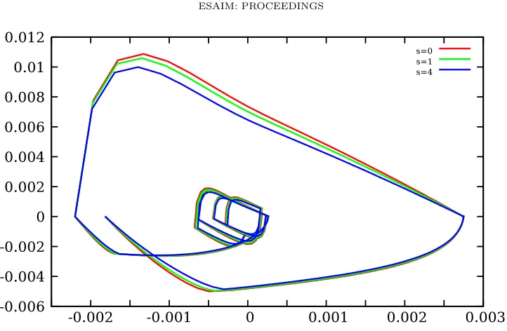
Figure 10. Flow (in m3_·_s−1_{) – Volume (in m}3_{) diagram for different values of}_k_{(see (30)).} k= 40.172 + 10(s−3), s= 0,2,4,6.

Figure 11. Flow (in m3_·_s−1_{) – Volume (in m}3_{) diagram for different values of} _θ _between θmin=−0.13636 and θmax= 0.10909 (given byxmin, xmax and formula (31)).

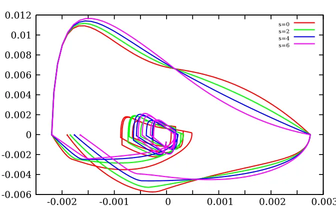
Comments :

• The sensitivity of the phase portrait of the coupled model seems to be more important for spring stiffness kand the parameterθthan for the resistancesRi.

(18)

Vec Value

0

1.1368e-05 2.2736e-05 3.41041e-05 4.54721e-05

5.68401e-05

6.82081e-05

7.95761e-05

9.09441e-05 0.000102312

IsoValue

-0.110444 -0.108277 -0.10611 -0.103943 -0.101776

-0.0996088

-0.0974417

-0.0952747

-0.0931076

-0.0909405

(19)

Figure 13. Flow (in m3_·_s−1_{) – Volume (in m}3_{) diagram for different values of}_Ra _{(see (31))} the resistances at the outlets on Γ7 and Γ8. Fori= 1..6,Ri =Rout on Γi and on Γ7 and Γ8, Ri =Rout×102(s−1)_.

Conclusions and perspectives

From a biological point of view, we note that we obtain some phase portraits that are comparable to the ones that can be found in [12]. The comparison of the results for different values ofθ,k, andRiare encouraging for a future better understanding of lung pathologies such as asthma (modification ofθ), or emphysema (modification ofk). Moreover, 2D simulations cannot reproduce all the 3D effects and 3D simulations have to be performed and exploited. Furthermore, note that other non linear spring models should maybe be developed in order to capture all the complexity of the phenomenon.

Concerning the numerical method, we have developed a method that could be easily implemented in any solver. There are two main drawbacks of our method. First, we can deal with the convection term only using an explicit method or a characteristic method (which has been chosen here). Secondly, this method is quite slow. A way to accelerate would be to choose a suitable resolution method for the Navier–Stokes problem such as a projection method to accelerate the solver (see [6, 14, 17]).

Acknowledgement. The authors want to thank Matteo Astorino, Laurent Boudin and Mourad Ismail for the very helpful scientific discussions which took place during Cemracs 2008 and after.

References

[1] D. N. Arnold, F. Brezzi, and M. Fortin. A stable finite element for the Stokes equations.Calcolo, 21(4):337–344 (1985), 1984. [2] L. Baffico, C. Grandmont, and B. Maury. Multiscale modelling of the respiratory track. HAL, 2008. Submitted, available at

http://hal.inria.fr/inria-00343629/en/.

[3] A. Ben-Tal. Simplified models for gas exchange in the human lungs.J. Theor. Biol., 238:474–495, 2006. [4] A-J. Chorin. Numerical solution of the Navier–Stokes equations.Math. Comp., 22:745–762, 1968.

[5] A-J. Chorin. On the convergence of discrete approximations to the Navier–Stokes equations.Math. Comp., 23:341–353, 1969. [6] A. Devys, C. Grandmont, B. Grec, and D. Yakoubi. Numerical method for non standard boundary conditions, work in progress. [7] C. A. Figueroa, K. E. Jansen, C. A. Taylor, and I. E. Vignon-Clementel. Outflow boundary conditions for three-dimensional

(20)

[8] L. Formaggia, J.-F. Gerbeau, F. Nobile, and A. Quarteroni. Numerical treatment of defective boundary conditions for the Navier-Stokes equations.SIAM J. Numer. Anal., 40(1):376–401 (electronic), 2002.

[9] C. Grandmont, Y. Maday, and B. Maury. A multiscale/multimodel approach of the respiration tree. InNew trends in continuum mechanics, volume 3 ofTheta Ser. Adv. Math., pages 147–157. Theta, Bucharest, 2005.

[10] C. Grandmont, B. Maury, and A. Soualah. Multiscale modelling of the respiratory track: a theoretical framework.ESAIM Proc., 23:10–29, 2008.

[11] F. Hecht, A. Le Hyaric, K. Ohtsuka, and O. Pironneau. Freefem++, finite elements software,http://www.freefem.org/ff++/. [12] S. Martin, B. Maury, T. Similowski, and C. Straus. Impact of respiratory mechanics model parameters on gas exchange

efficiency.ESAIM: PROCEEDINGS, 23, (2008) 30–47.

[13] M.S. Olufsen. Structured tree outflow condition for blood flow in larger systemic arteries.Am. J. Physiol., 276:257–H268, 1999. [14] L. Quartapelle. Numerical solution of the incompressible Navier–Stokes equations.International Series of Numerical

Mathe-matics, 113, 1993.

[15] A. Quarteroni, S. Ragni, and A. Veneziani. Coupling between lumped and distributed models for blood flow problems. Com-put.Visualization Sci., 4 (2):111124, 2001.

[16] A. Quarteroni and A. Veneziani. Analysis of a geometrical multiscale model based on the coupling of odes and pdes for blood flow simulations.Multiscale Model. Simul., 1, No.2:173–195, 2003.

[17] R. Rannacher. On Chorin’s projection method for the incompressible Navier–Stokes equations. Lecture Notes in Math., 1530:167–183, 1992.

[18] A. Soualah-Alilah.Modélisation mathématique et numérique du poumon humain. PhD thesis, Université Paris-Sud–Orsay, 2007.

[19] R. Temam. Navier–Stokes equations. theory and numerical analysis.Studies in Mathematics and its Applications, 2, 1977. [20] Alessandro Veneziani and Christian Vergara. An approximate method for solving incompressible Navier-Stokes problems with