S. Dellacherie, F. Dubois, S. Fauve, R. Gatignol, Editors
QUANTUM LATTICE ALGORITHMS: SIMILARITIES AND CONNECTIONS TO
SOME CLASSIC FINITE DIFFERENCE ALGORITHMS
Paul J. Dellar
1Abstract. Quantum lattice algorithms originated with the Feynman checkerboard model for the one-dimensional Dirac equation. They offer discrete models of quantum mechanics in which the complex numbers representing wavefunction values on a discrete spatial lattice evolve through discrete unitary operations. This paper draws together some of the identical, or at least unitarily equivalent, algorithms that have appeared in three largely disconnected strands of research. Treated as conventional numerical algorithms, they are all only first order accurate under refinement of the discrete space/time grid, but may be raised to second order by a unitary change of variables. Much more efficient implementations arise from replacing the evolution through a sequence of unitary intermediate steps with a short path integral formulation that expresses the wavefunction at each spatial point on the most recent time level as a linear combination of values at immediately preceding time levels and neighbouring spatial points. In one dimension, a particularly elegant reformulation replaces two variables at two time levels with a single variable over three time levels. The resulting algorithm is a variational integrator arising from a discrete action principle, and coincides with the Ablowitz–Kruskal–Ladik finite difference scheme for the Klein–Gordon equation.
1.
Introduction
Quantum lattice algorithms originated with Feynman’s checkerboard model for the Dirac equation that describes a spin-1/2 particle moving relativistically on a discrete space-time lattice with one spatial dimension [1]. Heisenberg [2] had previously developed a spatially discrete “Gitterwelt” (lattice world) theory. Carazza & Kragh[3] give a fascinating reconstruction of this theory, which was communicated almost entirely in unpublished correspondence.
Subsequent work has followed three parallel lines of development, frequently leading to identical, or at least unitarily equivalent, algorithms under the different names of quantum cellular automata, discrete time quantum walks, and “quantum lattice Boltzmann” algorithms. The first two strands emphasise algorithms for quantum computers, notablyO(√N) search algorithms. The last strand emphasises simulation of quantum phenomena using conventional digital computers by applying techniques used in the derivation of the hydrodynamic algo-rithms from the Boltzmann equation. They would be better described as “lattice Dirac algoalgo-rithms” as they have no connection to the quantum Boltzmann equation. All strands offers unitary and readily parallelisable algorithms that are free of the fermion-doubling problem that are commonly found in finite difference or finite element discretisations of quantum mechanical equations. In discrete quantum systems the finite-time evolu-tion operator replaces the Hamiltonian as the principle object of interest. Unitary evoluevolu-tion implies that the
1OCIAM, Mathematical Institute, Andrew Wiles Building, Radcliffe Observatory Quarter, Woodstock Road, Oxford OX2 6GG, UK
c
EDP Sciences, SMAI 2015
expectation of the evolution operator is itself conserved, offering an exact invariant of the discrete system that is consistent with the energy conservation property of the continuous system implied by Ehrenfest’s formula [4]. A fourth line of development treats the Schr¨odinger equation and its nonlinear extensions as reaction-diffusion equations for complex wavefunctions [5–7], and adapts standard lattice Boltzmann techniques for reaction-diffusion equations [8]. The target partial differential equation then describes slowly varying solutions on some manifold within an enlarged state space for a dissipative system, just as in lattice Boltzmann formulations for hydrodynamics. These formulations are thus neither unitary nor reversible, and will not be considered further. This paper is based on a tutorial presented at the Discrete Simulation of Fluid Dynamics conference, Yerevan, Armenia, 15–19 July 2013. It covers all three strands above, though devoting most attention to the develop-ment of second-order accurate quantum lattice algorithms for simulating the Dirac equation with a potential in multiple space dimensions. Such algorithms are finding new applications beyond quantum electrodynamics and laser-plasma interactions. The Dirac equation also offers a large-scale description of charge carriers within graphene, a two-dimensional hexagonal lattice of carbon atoms, with a vector potential arising from uneven strain within the lattice [9]. Other experimental replications of the Dirac equation use trapped ions in optical lattices. These analogous systems are bringing previously inaccessible phenomena from quantum electrody-namics such as Zitterbewegung and the Klein paradox within experimental and technological reach. A detailed description of a second-order one-dimensional algorithm, and early multi-dimensional algorithms, may be found in the thesis [10].
2.
The Dirac and Schr¨
odinger equations
The Dirac equation offers a quantum mechanical description of spin-1/2 particles such as electrons that is compatible with special relativity [11–14]. It may be written as the abstract Schr¨odinger equation
i∂tψ=Hψ (1)
in convenient “natural” units in which the speed of light c= 1 and the reduced Planck’s constant~= 1. The
wavefunctionψ= (ψ1, ψ2, ψ3, ψ4)Thas four components. The Hamiltonian is
H= (−iα· ∇+mβ−g1), (2)
wherem is the particle mass,g(x) is a time-independent scalar potential,1is the 4×4 identity matrix,β is a 4×4 matrix, andαis a vector of three 4×4 matrices such that α· ∇=αx∂
x+αy∂y+αz∂z. These matrices
may be written in block form as
αi=
0 σi σi 0
, β=
1 0 0 −1
, (3)
in which1 is now the 2×2 identity matrix. The off-diagonal blocks are the three Pauli spin matrices
σx=
0 1 1 0
, σy=
0 −i i 0
, σz=
1 0 0 −1
, (4)
which satisfy the relations [12–15]
σiσj =1δij+ iijkσk, (5)
whereijk is the alternating Levi-Civita tensor.
This Hamiltonian arose from Dirac’s efforts to construct an operator analogue of the relativistic energy-momentum relation E2 = m2+|p|2, in c = 1 units, in which p = −i∇ is the momentum operator. The
space-time symmetry expected in special relativity suggests that the Hamiltonian should be a first-order spatial differential operator, to match the single ∂t on the left hand side of (1), in contrast to the second-derivative
Laplacian that appears in the non-relativistic Schr¨odinger equation (see below). Naively, one expects the Hamiltonian to be related to E = ±p
4×4 matrix Hamiltonian let him construct such a square root that was linear inp, i.e.using only first-order spatial derivatives.
These two constraints, achieving compatibility with E2 = m2+|p|2, and using only first-order spatial
derivatives, thus imply not only the existence of quantum mechanical spin, through the appearance of the Pauli spin matrices above, but also the existence of both positive and negative energy states – the positron as well as the electron – arising from the positive and negative 2×2 blocks in theβ matrix.
Dirac’s construction just imposes a set of algebraic relations between theαandβ matrices,
αiαj+αjαi= 2δij, β2=1, αiβ+βαi= 0, (6)
analogous to the relations (5) between the three σ matrices. Any set of matrices satisfying these relations yields a representation of the abstract Dirac algebra. The Dirac equation may thus be written in many appar-ently different, but ultimately equivalent, forms. The concrete expressions for α and β given above, and the Hamiltonian (2), give what is commonly called the “standard representation” of the Dirac equation.
2.1.
From the Dirac to the Schr¨
odinger equation
The most convenient starting point for taking the non-relativistic limit is the Dirac equation for a free particle
(∂t+α· ∇)
ψ+ ψ−
=−imβ
ψ+ ψ−
(7)
in whichψ= (ψ+, ψ−)T has been split into two two-component pairsψ±. Equation (7) then separates into
∂tψ++σ· ∇ψ−=−imψ+, (8a) ∂tψ−+σ· ∇ψ+= imψ−. (8b)
The crossing over of ψ+ and ψ− in the σ· ∇ terms is due to the off-diagonal blocks being non-zero in theα
matrices. In the absence of spatial gradients, we find from (8a,b) that ψ+ oscillates in proportion to e−imt,
whileψ− oscillates in proportion toeimt.
Following Pauli [11] and Berestetskii et al. [13], we break the symmetry between ψ+ and ψ− by seeking
solutions whose time-dependence is close to oscillation in proportion toe−imt. This is equivalent to shifting the energy origin from 0 tom. Writing
ψ±(x, t) =φ±(x, t)e−imt (9)
and substituting into (8a,b) gives
∂tφ++σ· ∇φ−= 0, (10a)
∂tφ−+σ· ∇φ+= 2imφ−. (10b)
The algebraic right hand side now only affects theφ−variable. By analogy with the derivation of hydrodynamics
from moments of the Boltzmann equation, we refer to φ+ as the slow, or hydrodynamic, variable, and φ− as
the fast, or nonhydrodynamic, variable. The slowly-varying approximation
∂tφ−
2m
φ−, (11)
holds in the non-relativistic limit, which corresponds to the kinetic energy being much less than the rest energy. Making this approximation in (10b) allows us to solve (10b) for φ− in terms of the gradient of φ+,
φ−=− 1
2miσ· ∇φ
Substituting this relation into the evolution equation (10a) for φ+ leads to the one-dimensional Schr¨odinger
equation for a free particle in natural units,
i∂tφ+=−
1 2m∇
2φ+, (13)
since (σ·∇)(σ·∇) =∇2using a property of theσmatrices. As in the derivation of the Navier–Stokes equations
from kinetic theory, the derivation of the Schr¨odinger equation follows from eliminating the fast variableφ− to obtain a closed evolution equation for the slow variable φ+ alone [16, 17].
2.2.
The Foldy–Wouthuysen transformation
Foldy & Wouthuysen developed a more elegant theoretical approach to the non-relativistic limit [12, 18, 19]. They found the exact unitary transformation
ψ0=eiSψ, S=βα·pθ(|p|), tan 2|p|θ(|p|)
=|p|/m, (14) under which the Dirac Hamiltonian for a free particle becomes
HNW=βpm2+|p|2. (15)
This Hamiltonian is the natural operator version of the relation E = pm2+|p|2 for a relativistic particle,
in which p is simply the momentum vector, whose components are numbers, rather than the momentum operator. The subscript NW indicates that HNW is the Hamiltonian in the Newton–Wigner representation.
This representation decouples the four components of the transformed wavefunction into two independent pairs:
i∂t
ψNW+ ψNW−
=HNW
ψNW+ ψNW−
=⇒ i∂tψNW±=±
p
m2+|p|2ψ
NW±. (16)
For plane wave solutions with momentump, the pairsψNW± thus correspond to energy and momentum
eigen-states with energies±p
m2+|p|2 respectively. Approximating the Hamiltonian in the Newton–Wigner
repre-sentation for solutions that vary slowly in space (|p| m) gives
HNW=βm
1 + 1 2
|p|2 m2 +· · ·
. (17)
Truncating after the|p|2/m2 term gives the usual Schr¨odinger operator|p|2/(2m) for each of the two blocks,
with a superimposed constant potential m that creates a phase rotation proportional to exp(±imt) in the wavefunctionsψNW±.
Moreover, the position operatorxNWin the Newton–Wigner representation satisfies the classical relation for a free particle,
d
dtxNW=vNW≡β p p
m2+|p|2. (18)
This is in stark contrast to the velocity operator in the original Dirac–Pauli representation, whose eigenvalues are ±c in SI units. This is responsible for the zitterbewegung or “trembling motion” of the expectation of the position operator in this representation.
However, the Foldy–Wouthuysen transformation sacrifices the locality of the Dirac HamiltonianH=βm+α· p. It replaces a first order hyperbolic system of partial differential equations with a system involving the spatially non-local operator pm2+|p|2 defined by its Fourier transform. The Foldy–Wouthuysen transformation is
expansion in 1/c. Theminimal coupling replacement ofpbyp−qAin the presence of a magnetic field holds in the original Dirac–Pauli representation, but not in the Newton–Wigner representation. The study of the Foldy–Wouthuysen and related transformations, such as the Douglas–Kroll–Hess expansion, remains active in quantum chemistry as part of many-electron theories for atoms and molecules [20].
2.3.
The one-dimensional Dirac equation
We consider solutions in which ψonly depends on z andt. Equation (1) then decouples into two separate subsystems, ∂t ψ1 ψ3
+∂z
ψ3 ψ1
=−im
ψ1 −ψ3
, ∂t
ψ2 ψ4
−∂z
ψ4 ψ2
=−im
ψ2 −ψ4
. (19)
These two subsystems describe the evolutions of states with different spins. They decouple due to the absence of spin-changing processes in the one-dimensional Dirac equation for a free particle. Each subsystem may be rewritten in matrix form as
∂t Φ+ Φ− + 0 1 1 0 ∂z Φ+ Φ−
=−im
Φ+ −Φ−
, (20)
by writing Φ+=ψ
1and Φ−=ψ3for the first subsystem, or Φ+ =ψ2and Φ− =−ψ4for the second subsystem.
Following the standard theory of hyperbolic systems, we diagonalise the matrix appearing in (20) as
0 1 1 0
=U†
1 0 0 −1
U, (21)
using the unitary matrix
U=
1/√2 1/√2 −i/√2 i/√2
=
1 0 0 −i
C, (22)
which is a diagonal multiple of the Hadamard transformation matrix Cdefined in (28) below. Equations (20) may thus be rewritten as
∂tu+∂zu = md, (23a)
∂td−∂zd = −mu. (23b)
The extra diagonal matrix with the−i coefficient in (22) allows this system to be written with real coefficients. The left hand sides now comprise a hyperbolic system in diagonal form. The variablesuanddare the Riemann invariants [21] of the hyperbolic system defined by the left hand side of (20). They are related to Φ± by the unitary transformation u d =U Φ+ Φ− , (24)
and they propagate along the two sets of characteristics (z, t) = (z0±s, t0+s) parametrised bys. For example,
(23a) becomes du/ds = md along the + characteristic, while (23b) becomes dd/ds = −mu along the − characteristic,
3.
Quantum algorithms on a one-dimensional lattice
3.1.
Discrete time quantum walks
Grover’s [26, 27] quantum search algorithm locates one marked item from amongN items inO(√N) steps by simulating a discrete time approximation to a Schr¨odinger equation with an attractive potential localised at the marked item. Childs et al.’s [28] graph traversal algorithm simulates a discrete time approximation to a Schr¨odinger equation whose Hamiltonian is a scaled adjacency matrix of the graph. The introduction below follows the review of Ambainis [29]. Other reviews include those by Kempe [30] and Kendon [31].
In the classical discrete time random walk on the line, at each time step we move left with probability 1/2, and right with probability 1/2. The natural quantum counterpart considers a basis of states|niforn∈Zwith
the transition rule
|ni →a|n−1i+b|ni+c|n+ 1i (25) at each step. If one considers an integer lattice with a scalar complex amplitude ψi at each point i, one may
think of|nias denoting the state in whichψn = 1 andψi= 0 for i6=n. The set of|niforn∈Zthus form a
basis for the vector space of complex amplitudes on the lattice. The update rule (25) extends by linearity into an infinite set of linear equations between the coefficientsψi before and after each timestep.
However, Meyer [25] showed that this transition rule is only unitary if one ofa, b, c has unit modulus while the other two vanish,i.e.the solutions are|a|= 1,b= 0,c= 0 and permutations. Up to an unimportant global phase, the only unitary operations are deterministic shifts in either direction and the identity operation. This is essentially because the inverse of a general tridiagonal matrix is a full matrix, not another tridiagonal matrix. Meyer [25] identified the very limited subset of tridiagonal matrices that satisfyU−1=U†.
This difficulty may be resolved by enlarging the state space to comprise two linearly independent states |n,−1i and |n,1i at each n ∈ Z. Each lattice pointi now holds two complex amplitudes ψ+i and ψ
− i . The
quantum element then arises through the creation of superpositions.
The one-dimensional discrete time quantum walk algorithm on the line comprises two steps:
• A “coin flip” transformationC,
C|n,−1i=a|n,−1i+b|n,1i, C|n,1i=c|n,−1i+d|n,1i, (26)
• followed by a shiftS,
S|n,−1i=|n−1,−1i, S|n,1i=|n+ 1,1i. (27)
Each step of the walk corresponds to applyingSC. The most comon choice for the matrixCis the Hadamard transformation
a b c d
=
1/√2 1/√2 1/√2 −1/√2
. (28)
ApplyingCtakes|n,−1ito √1
2|n,−1i+ 1
√
2|n,1i, and takes|n,1ito 1
√
2|n,−1i − 1
√
2|n,1i. ApplyingCto either
basis state thus gives a superposition of the two basis states, each of which will be observed with probability 1/2. This is the sense in which applyingCcorresponds to a coin flip.
Shenvi et al. [32] showed that the discrete time quantum walk achieves the same asymptotic performance as Grover’s [26, 27] quantum search algorithm. Lovett et al. [33] later showed that the discrete time quantum walk can implement the universal quantum gate set, following Childs’ [34] earlier proof of the equivalent result for the continuous time quantum walk. Ryan et al. [35] experimentally demonstrated eight steps of a discrete time quantum walk over three points using an NMR-based quantum computer.
A more general quantum walk uses a biased coin. It replaces the Hadamard matrix (28) with
Cθ=
cosθ −i sinθ −i sinθ cosθ
for a rotation angleθ∈(0, π/2). The composition ofCfollowed byS defines the unitary mapping
ψ+(n, τ + 1) = cosθ ψ+(n−1, τ)−i sinθ ψ−(n−1, τ), (30a) ψ−(n, τ + 1) = cosθ ψ−(n+ 1, τ)−i sinθ ψ+(n+ 1, τ), (30b) where n, t ∈ Zare discrete space and time coordinates. This algorithm is identical to a quantum lattice gas automaton introduced by Meyer [25, 36].
Strauch [37] reviewed and extended results on the behaviour of this algorithm in the continuum limit. The continuum limit withθ→0 yields the one-dimensional Dirac equation. This result is originally due to Feynman, and gives his checkerboard path integral formulation for the one-dimensional Dirac equation for a particle with mass controlled by θ [1]. The precise limit arises from creating a space-time lattice with z =j∆t, t =n∆t, putting θ =m∆t for a particle of mass m, and taking the limit ∆t →0 at fixed z andt. Conversely, taking θ→π/2 in (30a,b) yields the one-dimensional continuous time quantum walk [38]
i∂tψ(n, t) =−γ{ψ(n+ 1, t)−2ψ(n, t) +ψ(n−1, t)}. (31)
This is recognisable as a spatial finite-difference approximation to the one-dimensional Schr¨odinger equation for a free particle. The constantγ sets the speed γ/2 at which local maxima in |ψ|2 propagate in the continuum
limit.
3.2.
Quantum cellular automata
The discrete time quantum random walk is just one example of the broader class of quantum cellular au-tomata and quantum lattice gases [25, 36, 39–41]. These systems replace the Boolean variables of classical cellular automata with complex amplitudes, allowing the state of the quantum automaton to be a superposi-tion of the states of the classical automaton. However, only a small subset of update rules produce unitary evolution. For example, the only unitary evolution that may be obtained from the quantum analogs (25) of the common one-dimensional nearest-neighbour cellular automata is a deterministic shift with a constant global phase multiplication (see previous section). An early general formulation for quantum cellular automata by Watrous [42] was later found to allow signal propagation with arbitrarily large velocities, so more restrictive axiomatic formulations with a causality property have been pursued since [43, 44]. Shakeel and Love [45] give a recent review.
Yepez [46] extended Feynman’s one-dimensional path integral formulation to a quantum lattice gas algorithm for the three-dimensional Dirac equation, and Yepez [47] gives a comprehensive exposition of quantum lattice gas algorithms for this and other physical systems. Yepez et al. [48] have performed very large-scale, up to 50763
points, simulations of the Gross–Pitaevskii (nonlinear Schr¨odinger) equation using a 2-component quantum lattice gas automata in the diffusive scaling regime in which ∆x∼and ∆t∼2. This is the same scaling that
leads from the Boltzmann equation directly to the incompressible Navier–Stokes equations in the small Mach number limit at fixed Reynolds number. It was adopted by Inamuro et al. [49] in a lattice Boltzmann context, following earlier work in continuum kinetic theory collected in the book by Sone [50].
3.3.
The “quantum lattice Boltzmann” algorithm
The hydrodynamic lattice Boltzmann equation may be derived from the discrete Boltzmann PDE through an integration along characteristics [51]. One may apply the same approach to the one-dimensional Dirac equation (23a,b) with a scalar potential,
∂tu+∂zu=md+ igu, ∂td−∂zd=−mu+ igd. (32)
for a timestep ∆tgives
u(z+ ∆z, t+ ∆t)−u(z, t) =12m∆t{d(z+∆z, t+ ∆t) +d(z, t)}
+12i∆t{g(z+ ∆z, t+ ∆t)u(z+ ∆z, t+ ∆t) +g(z, t)u(z, t)}, (33a) d(z−∆z, t+ ∆t)−d(z, t) =−1
2m∆t{u(z−∆z, t+ ∆t) +u(z, t)}
+12i∆t{g(z−∆z, t+ ∆t)d(z−∆z, t+ ∆t) +g(z, t)d(z, t)}. (33b) The left hand sides are exact, while the algebraic terms on the right hand sides have been approximated using the trapezoidal rule. We can now put ∆z= ∆t since the PDE system (32) is written inc= 1 units.
The above pair of algebraic equations is not closed, becaused(z+∆t, t+ ∆t) appears on the right hand side of (33a), while d(z−∆t, t+ ∆t) appears on the left hand side of (33b). Similarly, u(z−∆z, t+ ∆t) appears on the right hand side of (33b), whileu(z+∆t, t+ ∆t) appears on the left hand side of (33a). The “quantum lattice Boltzmann” (QLB) algorithm [52, 53] alters the locations at which uand dare evaluated, and also the location at which the potentialg is evaluated, to obtain the closed pair of algebraic equations
u(z+ ∆z, t+ ∆t)−u(z, t) = 12m∆t{d(z−∆z, t+ ∆t) +d(z, t)}
+12i∆tg(z, t){u(z+ ∆z, t+ ∆t) +u(z, t)}, (34a) d(z−∆z, t+ ∆t)−d(z, t) =−1
2m∆t{u(z+∆z, t+ ∆t) +u(z, t)}
+1
2i∆tg(z, t){(z−∆z, t+ ∆t) +d(z, t)}. (34b)
Solving these two linear equations determines
u(z+ ∆z, t+ ∆t) = a(z, t)u(z, t) +b(z, t)d(z, t), (35a) d(z−∆z, t+ ∆t) = a(z, t)d(z, t)−b(z, t)u(z, t), (35b) with coefficients
a(z, t) = 1−
1 4∆t
2(m2
−g(z, t)2)
1−ig(z, t)∆t+14∆t2(m2−g(z, t)2), b(z, t) =
m∆t
1−ig(z, t)∆t+14∆t2(m2−g(z, t)2). (36) These coefficients satisfy |a|2+|b|2 = 1 and ab∗ = a∗b, so the right hand sides of (35a,b) are equivalent to
multiplying the vector (u, d)T by a unitary matrix. Meyer [25] showed that this algorithm for a free particle is
unitarily equivalent to the discrete time quantum walk described above.
4.
Convergence properties
The above algorithm, in its three different guises, evolves the wavefunction values u and d on a discrete space/time lattice through a sequence of unitary operations. However, it provides only a first-order accurate approximation to the one-dimensional Dirac equation. That the accuracy is only first order may most easily be seen from the approximation ofu(z−∆z, t+∆t) byu(z+∆z, t+∆t), and ofd(z+∆z, t+∆t) byd(z−∆z, t+∆t) in the derivation in Sec. 3.3. Alternatively, the first-order accuracy is due to the approximation of the simultaneous evolution through both spatial derivatives and algebraic terms by the sequential evolution under these terms separately, as expressed by theSCpair in Sec. 3.1.
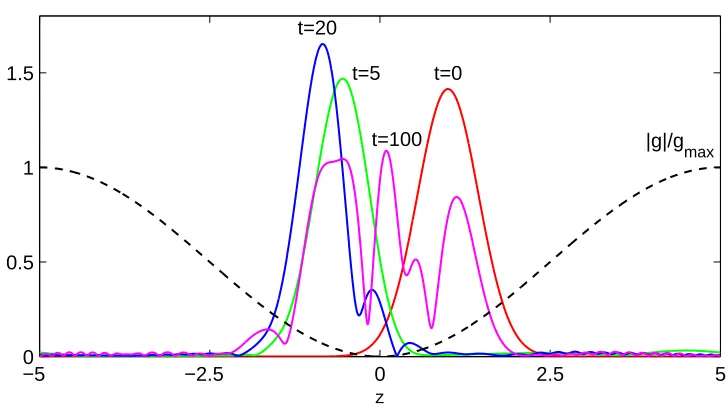
Figure 1 shows the resulting solution for a particle with mass m = 20 in the periodic potential g(z) = −20 sin2(πz/10) on the intervalz∈[−5,5) with periodic boundary conditions. The initial conditions
Φ+0 = 1 (2π∆2
0)1/4
exp
−(z−z0) 2
4∆2 0
+iκ(z−z0)
−50 −2.5 0 2.5 5 0.5
1
1.5 t=0
t=100 t=20
t=5
|g|/gmax
z
Figure 1. Evolution of|Φ+|for an initial Gaussian wavepacket centred atz= 1 in a sinusoidal potential (shown dotted and normalised to a maximum of 1).
and Φ−0 = 0 approximate a non-relativistic wavepacket centred around z0 = 1 with spread ∆20 = 0.1 and
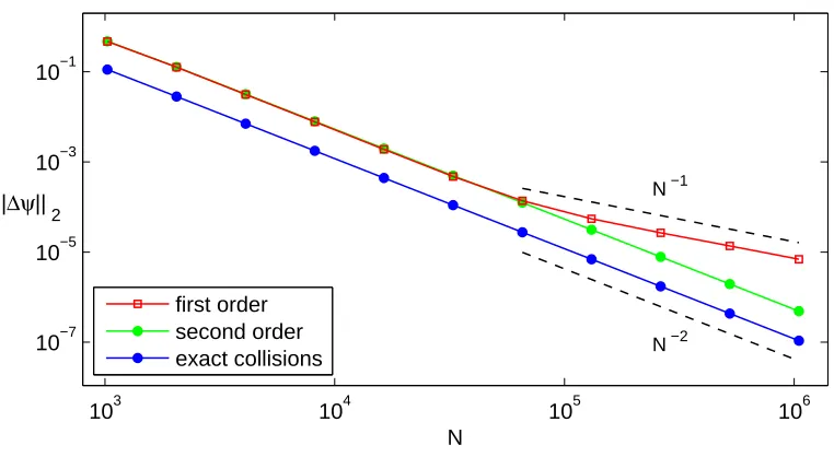
momentum κ = 0.5. The plot also shows the spatial variation of the potential g(z), which is an attactive potential for the Φ+ component. Figure 2 shows the errors inψ= (u, d)Tcomputed using the Succi–Benzi QLB
scheme, and the two second-order schemes described below. The quantity plotted is the root-mean-square error
||∆ψ||2= "
1 N
N
X
i=1
ui−urefi
2
+di−diref
2 #1/2
(38)
relative to an expotentially accurate reference solution (uref
i , diref) on the same spatial lattice. As expected, the
standard quantum lattice algorithms, and the unitarily equivalent Succi–Benzi QLB scheme, are only first order accurate, while the two improved schemes described below are second order accurate.
4.1.
Computation of reference solutions
If we represent u and d by vectors of values at a uniformly spaced set of points x = {x1, . . . , xN}, u =
{u1, . . . , uN},d={d1, . . . , dN}, with periodic boundary conditions, we may write a semi-discrete approximation
to the one-dimensional Dirac equation in matrix form as
d dt
u d
=E
u d
, where E=
−D−G m1 −m1 D−G
. (39)
The 2N×2N evolution matrixE is made up ofN×N blocks involving the Fourier differentiation matrixD, the identity matrix1, and the diagonal matrix G= diag(g(x1), . . . , g(xN)) whoseith entry isg(xi).
The solution of this matrix ODE system with initial conditions u0 andd0 is
u(t)
d(t)
= exp(tE)
u0 d0
103 104 105 106 10−7
10−5 10−3 10−1
N −2 N −1
N ||∆ψ||
2
first order second order exact collisions
Figure 2. Convergence in the discrete`2 norm ofψ= (u, d)Tatt= 100 towards an
exponen-tially accurate reference solution with increasing numbers of gridpointsN.
where the matrix exponential is defined by the convergent series
exp(tE) =
∞
X
n=0
(tE)n
n! . (41)
The efficient and accurate computation of the matrix exponential has been the subject of two noteworthy reviews by Moler & van Loan [54, 55]. The most common approach uses scaling and squaring, or repeated application of the property
exp(tE) = exp 1
2tE 2
. (42)
We determine an integerrsuch that 2−rtEis small enough for a truncation of the series (41) to give sufficient
accuracy with a reasonable number of terms, and then square the resulting matrix r times. Greater accuracy in finite precision arithmetic may be obtained by using a Pad´e approximation for exp(2−rtE) in place of a
truncated power series [56, 57].
The reference solutions used in the convergence plot were computed using 512 Fourier collocation points. The matrixE is small enough for a direct computation of exp(tE) by scaling and squaring using theexpokit package [56], while the Fourier differentiation matrix provides exponential accuracy. The reference solution valuesurefi anddiref were constructed by zero-extending the Fourier coefficients to form a Fourier series on the fine grid, then computing an inverse FFT on the fine grid.
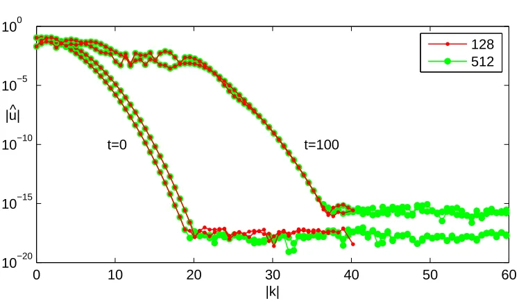
The Fourier transform of the Gaussian initial conditions (37) decays rapidly like exp(−∆20k2) with increasing |k|. Figure 3 shows the moduli of the Fourier coefficients ˆu(kn, t) forkn= 2πn/10 for these initial conditions,
0 10 20 30 40 50 60 10−20
10−15 10−10 10−5 100
t=0 t=100
|k| |u|^
128 512
Figure 3. The rapid decay of |uˆ(k, t)| with increasing |k| persists from t = 0 to t = 100.
The spectral solutions computed by matrix exponentiation using 128 and 512 Fourier modes are thus close to indistinguishable. The two different curves for each tarise from positive and negativek.
5.
Plane wave solutions
One may also investigate the accuracy of these discrete algorithms from the behaviour of individual Fourier modes, following the approach of Strauch [37] for quantum random walks, or the equivalent von Neumann approach for finite difference schemes [58, 59]. The spatial Fourier transform of the one-dimensional Dirac equation for a free particle may be written as
i∂t
uˆ ˆ d
=Hk
uˆ ˆ d
, (43)
where ˆuis the spatial Fourier transform ofu,
ˆ
u(k, t) =√1 2π
Z ∞
−∞
u(z, t)e−ikzdz, (44)
and the Hamiltonian is the 2×2 matrix
Hk =
k im −im −k
=kσz+mσy. (45)
The solution to (43) with initial conditions ˆu0 and ˆd0 may be written as
uˆ ˆ d
= exp(−itHk)
uˆ 0
ˆ d0
. (46)
The exponential of the Hamiltonian is
with Ω =√m2+k2, using properties of the Pauli spin matrices.
5.1.
Plane wave solutions of the discrete algorithm
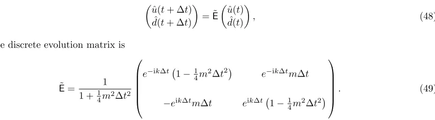
In contrast, substitutingu(z, t) = ˆu(t)eikz andd(z, t) = ˆd(t)eikz into the discrete algorithm (35) yields
uˆ(t+ ∆t) ˆ
d(t+ ∆t)
= ˜E uˆ(t)
ˆ d(t)
, (48)
where the discrete evolution matrix is
˜
E= 1
1 + 14m2∆t2
e−ik∆t 1−1 4m
2∆t2
e−ik∆tm∆t
−eik∆tm∆t eik∆t 1−1 4m
2∆t2
. (49)
The coefficients of the matrix ˜Eagree up to and including terms of O(∆t) with those of the exact evolution matrixE= exp(−itHk) defined above. This is consistent with the observed first order global accuracy.
The eigenvalues of ˜Emay be written as ˜λ±= exp(±iΩ∆˜ t) where
˜ Ω = 1
∆tcos
−1 (
cos (k∆t) 1−
1 4m
2∆t2
1 +14m2∆t2 !)
= Ω−m
2(m2+ 2k2)
12Ω ∆t
2+O(∆t4). (50)
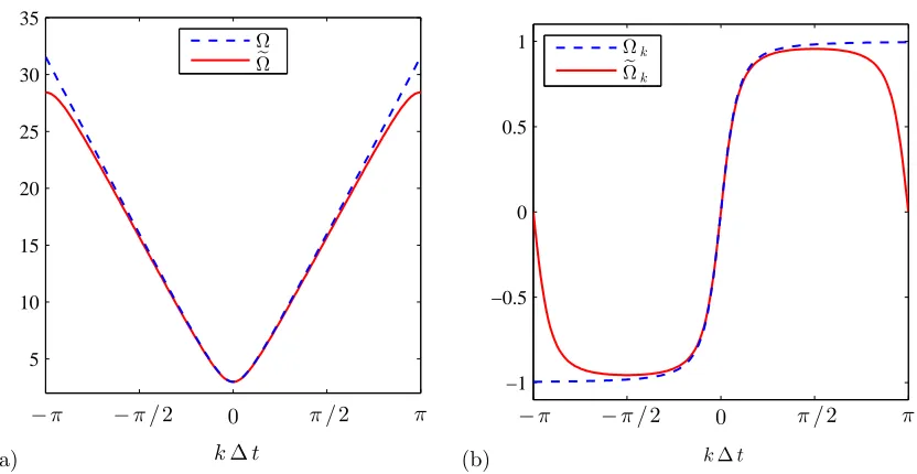
The discrete eigenvalues thus differ from the eigenvalues of the exact Dirac evolution matrix by anO(∆t2) error. Figure 4(a) compares ˜Ω and Ω for the parametersm= 3 and ∆t = 0.1. The productm∆t is relatively large, to make differences between Ω and ˜Ω easily visible.
The group velocity for waves in the numerical scheme is
∂Ω˜ ∂k =
sin(k∆t) sin( ˜Ω∆t)
1−1 4m
2∆t2
1 + 14m2∆t2 !
, (51)
while the group velocity for waves in the Dirac equation is∂Ω/∂k =k/Ω. These two expressions are plotted in Fig. 4(b). The numerical group velocity has the same sign as the true group velocity everywhere except at the points k∆t =±π where the numerical group velocity vanishes. The discrete frequency ˜Ω thus varies monotonically over the intervals 0 ≤ k∆t ≤ π and −π ≤k∆t ≤ 0, so the quantum lattice algorithm is free of the fermion doubling problem that affects many finite difference and finite element schemes for the Dirac equation.
5.2.
Fermion doubling
The fermion doubling problem may be illustrated with the first order wave equationut+uz= 0, as obtained
in Sec. 2.3 for a massless (m= 0) particle. Approximating the spatial derivativeuz using the natural centred
finite difference scheme on a spatial lattice with pointszn =n∆z, while leaving time continuous, gives
d dtun+
un+1−un−1
2∆z = 0. (52)
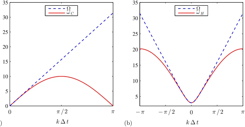
This equation has plane wave solutionsun(t) = exp(i(kn∆z−ωt)) withω= sin(k∆z)/∆zas shown in figure 5(a)
(a)
5 10 15 20 25 30 35
k∆t
−π −π/2 0 π/2 π Ω
e
Ω
(b)
−1 −0.5 0 0.5 1
k∆t
−π −π/2 0 π/2 π Ωk
e
Ωk
Figure 4. (a) Discrete and continuous dispersion relations for the parameters m = 3 and
∆t= 0.1. (b) Discrete and continuous group velocities∂Ω/∂kand∂Ω˜/∂kfor the same param-eters.
origin of the name “fermion doubling”. Moreover, the group velocitycg= dω/dkis positive fork∆z∈(0, π/2)
and negative fork∆z∈(π/2, π).
The second set of solutions to the dispersion relation appear because the spatial stencil is twice as wide as the spacing ∆z between lattice points. The natural solution is to reduce the width of the stencil by using the upwind differencing formula
d dtun+
un−un−1
∆z = 0. (53)
This gives the complex dispersion relation
ω= 2 ∆zsin
k∆z 2
exp
−ik∆z
2
, (54)
with expansion
ω=k−1 2ik
2∆z−1
6k
3∆z2+· · · . (55)
The first imaginary term gives a diffusive decay of the solution over time, as a consequence of the upwind dif-ferencing. This is incompatible with unitary and time-reversible evolution in a quantum system. The analogous downwind differencing (un+1−un)/∆z would give exponential growth due to an effective negative diffusivity.
Nielsen & Ninomiya [60–62] formalised these concrete examples into a “no-go” theorem for the non-existence of a spatial discretisation that gives unitary evolution (no spurious growth or decay) in continuous time, and a 1-to-1 relation between frequency and wavenumber.
The quantum lattice algorithms avoid these difficulties by discretising both space and time, so that (53) becomes
un(t+ ∆t)−un(∆t)
∆t +
un(t)−un−1(t)
∆z = 0, (56)
and synchronising the space and time steps (∆z= ∆t) so that (56) becomesun(t+ ∆t) =un−1(t), which is the
(a)
0 5 10 15 20 25 30 35
k∆t
0 π/2 π
Ω ωC
(b)
5 10 15 20 25 30 35
k∆t
−π −π/2 0 π/2 π Ω
ωH
Figure 5. (a) Dispersion relation for the centred finite difference approximation to the wave
equation showing fermion doubling. (b) Dispersion relation for Heisenberg’s Gitterwelt with parametersm= 3 and ∆t= 0.1. The numerical dispersion relations are shown as solid curves, and those of the underlying PDEs are shown dotted.
5.3.
Heisenberg’s Gitterwelt
Heisenberg [2] proposed the spatial discretisation
d2
dt2un−
un+1−2un+un−1
∆z2 +m 2u
n= 0, (57)
for the Klein–Gordon equation. This semi-discrete equation has dispersion relation
ω2=m2+ (2/∆z)2sin2(k∆z/2), (58)
which is shown in figure 5(b) for the parameters m = 3 and ∆z = 0.1. The effective mass of the particle represented by a solution of this dispersion relation is determined by dcg/dk= d2ω/dk2. This gives the rate at
which the group velocitycg changes with the momentumk, and hence the reciprocal of the mass. Atk= 0 the
curvature d2ω/dk2 = 1/m as expected, while d2ω/dk2 ∼ −∆z/2 for k=π/∆z if m∆z 1. The dispersion
relation near k = π/∆z then corresponds to that of a particle with the opposite charge and a much larger effective mass [2, 3].
Heisenberg’s dispersion relation shows some qualitative similarities with the dispersion relation for the quan-tum lattice algorithm shown in figure 4, notably thatω is a monotonic function of k. However, the curvatures neark= 0 andk=π/∆z are different in magnitude, and time is continuous rather than discrete.
6.
A second-order accurate one-dimensional algorithm
The discrete algebraic system (33a,b) may be extended into a second-order accurate algorithm using a change of variables equivalent to the fi tofi introduced by He et al. [51] in their second-order accurate derivation of
introduced by Dellar [63] for hydrodynamic lattice Boltzmann algorithms using Strang [64] splitting is simpler and more natural in a quantum context, as it guarantees that the overall algorithm is unitary.
The idea of splitting a unitary evolution into a product of simpler unitary operators is natural in quantum computation [46]. However, the quantum computation literature is primarily concerned with achieving any kind of convergence for algorithms adapted to quantum computers, rather than achieving second-order convergence with algorithms for conventional digital computers.
Separating the one-dimensional Dirac equation with a scalar potential into two operators,
∂t
u d
=
−∂z 0
0 ∂z
u d
, ∂t
u d
=
ig m −m ig
u d
, (59)
is equivalent to splitting the Hamiltonian into its spatial derivative and algebraic parts. The solutions to the two parts may be written using the operators
S=
exp(−∆t∂z) 0
0 exp(∆t∂z)
, C= exp
∆t
ig m −m ig
=eig∆t
cosm∆t sinm∆t −sinm∆t cosm∆t
. (60)
The exp(±∆t∂z) coefficients on the diagonal ofScome from the identity
ψ(z+ ∆z) =
∞
X
n=0
∆zn
n! (∂
n zψ)
z
= exp(∆z∂z)ψ
z
, (61)
and ∆z=±∆t in natural units. Combining theS andCoperators gives the update rule
ψ(t+ ∆t) =SCψ(t), (62)
whereψ(t) = (u(0, t), . . . , u(n∆z, t), d(0, t), . . . , d(n∆z, t))Tis the vector ofuanddvalues at lattice points. This
is the form that appears in the discrete time quantum walks of Sec. 3.1.
Instead of using the above exact expression, we may approximate the exponential of the collision (or coin flip) operator using the Crank–Nicolson form
1−1 2i∆tHm
1+12i∆tHm
−1
= exp(−i∆tHm) +O(∆t3). (63)
The expression on the left hand side is unitary wheneverHmis Hermitian. It defines
˜
C= 1
1−i∆tg−1 4∆t
2(g2−m2)
1 +1
4∆t
2(g2−m2) m∆t −m∆t 1 + 14∆t2(g2−m2)
, (64)
which gives the same unitary and second-order accurate approximation to the algebraic terms that appears in the quantum lattice Boltzmann algorithm [52].
Either algorithm is unitary, but the combinationsSCandSC˜ are only first order accurate due to the splitting error between the non-commuting operatorsSandCor ˜C. We may construct a second-order accurate algorithm using Strang’s [64] splitting formula
ψ(t+ ∆t) =C1/2SC1/2ψ(t) (65) or the equivalent using ˜Cinstead ofC. Applying this algorithm forntimesteps gives
ψ(t+n∆t) =C1/2SC1/2C1/2SC1/2· · ·C1/2SC1/2ψ(t), (66) and we may combine adjacent pairs usingC1/2C1/2=Cto obtain
The integration along characteristics approach leads naturally to collisions preceding streaming, so we rewrite the above as
ψ(t+n∆t) =C1/2(SC)nC−1/2ψ(t), (68) using the identityC1/2=CC−1/2. We thus recover what looks like the previous first-order splitting,
˜
ψ(t+n∆t) = (SC)nψ˜(t), (69)
but applied to the transformed wavefunctions
˜
ψ=C−1/2ψ, ψ=C1/2ψ.˜ (70)
This transformation raises the accuracy from first order to second order in ∆t. The operators C±1/2 are applied only once each per computation, not once per timestep, so we may tolerate O(∆t2) errors in C±1/2
while preserving global second-order accuracy. For example, approximatingC1/2≈ 1
2(1+C) leads to the same fi →fi transformation introduced by He et al. [51] for the hydrodynamic lattice Boltzmann algorithm [63].
However, algorithms for quantum mechanics should be unitary, which 12(1+C) is not, so we use either the exact formula
C±1/2= exp
±1 2∆t
ig m −m ig
=eig∆t/2
cosm∆t/2 ±sinm∆t/2 ∓sinm∆t/2 cosm∆t/2
. (71)
or the Crank–Nicolson approximation
˜
C±1/2= 1∓1 4i∆tHm
1±1
4i∆tHm −1
. (72)
Either transformation raises the previous first-order algorithms to second-order accuracy, as shown in figure 2. In terms of our earlier Fourier analysis, we replace ˜E with C1/2EC˜ −1/2. This similarity transformation leaves the eigenvalues, which were already second-order accurate, unchanged, but corrects the O(∆t) terms in the eigenvectors to agree with the eigenvectors of the exact evolution operator E.
7.
A second-order accurate algorithm with exact collisions
While the formulation (3.3) with its aandbcoefficients arises naturally from integrating the complete one-dimensional Dirac equations along characteristics, the splitting approach in (6) shows that one could equally well employ the exact solution (60) of the decoupled system (59) involving onlymandginstead of the second-order Crank–Nicolson approximation (64). This gives the alternative algorithm
u(z+ ∆z, t+ ∆t) =eig(z)∆t(cos(m∆t)u(z, t) + sin(m∆t)d(z, t)), (73a) d(z−∆z, t+ ∆t) =eig(z)∆t(cos(m∆t)d(z, t)−sin(m∆t)u(z, t)), (73b) for a time-independent potential. For a free particle, this is equivalent to replacingmwith an effective numerical mass
˜ m= 2
∆ttan 1
2m∆t
∼m
1 + 1 12m
2∆t2+ 1
120m
4∆t4+· · ·
. (74)
The tangent half-angle formulae then imply
˜ m∆t 1 + ˜m2∆t2
/4 = sin(m∆t), and
1−m˜2∆t2 /4 1 + ˜m2∆t2
/4 = cos(m∆t), (75)
In terms of computational cost, cos(m∆t) and sin(m∆t) are constants that may be precomputed. This just leaves the evaluation of eig(z)∆t, while the Crank–Nicolson matrix requires the reciprocal of the complex denominator 1−ig(z, t)∆t+14∆t2(m2−g(z, t)2). On modern hardware these two operations are of comparable cost, and both are typically negligible compared with loading and storing data. The complex exponential is usually best evaluated as cos(g(z)∆t) + i sin(g(z)∆t), due to the availability of fast routines to compute simultaneously both sin and cos of a real argument.
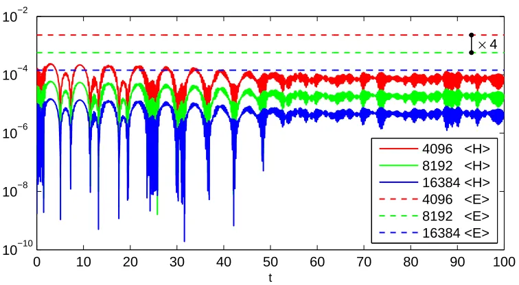
In concrete implementations on an Nvidia K20c GPU with error correcting code (ECC) memory disabled, both algorithms offer about 2200 million lattice updates per second using 64 bit floating point arithmetic. This corresponds to a useful memory bandwidth of 136 GBytes per second, based on the complex u and d being read and written once per lattice point, and the real gbeing read once. The algorithm using exponentiation is about 3% slower, but the resulting errors are about 4 times smaller, as shown by the lower blue line in figure 2. Again, one needs to pre- and post-process usingC±1/2 to achieve second-order accuracy.
This is the quantum equivalent of the hydrodynamic lattice Boltzmann algorithm with exact collisions in [63]. However, the standard hydrodynamic lattice Boltzmann algorithm relies upon a cancellation between the splitting error and the error in the Crank–Nicolson approximation of collisions to achieve grid-scale Reynolds numbers above unity. The errors in the hydrodynamic part of the solution are larger if one uses the exact solution of the collision step in place of the Crank–Nicolson approximation. In particular, the Crank–Nicolson approximation yields the correct hydrodynamic viscosity even for ∆t τ, while the algorithm with exact collisions gives an incorrect viscosity unless ∆t < τ.
8.
Multiple space dimensions
The quantum lattice Boltzmann approach was inspired by the structural similarities between the Dirac equation in the form
(∂t+α· ∇)ψ= i(g1−mβ)ψ, (76)
and the discrete Boltzmann equation
(∂t+ξi· ∇)fi= n
X
j=0
Ωij
fj−f
(0) j
, (77)
that forms the basis of hydrodynamic lattice Boltzmann algorithms. Both are linear, symmetric, hyperbolic systems with algebraic source terms. However, the discrete Boltzmann equation (77) is highly unusual among multi-dimensional hyperbolic systems in possessing one-dimensional characteristic curves of the form (x, t) = (x0+sξi, t0+s) with parameters. Writing (77) out in full gives
∂t+
ξ0x 0 · · · 0
0 ξ1x · · · 0
..
. ... . .. ... 0 0 · · · ξnx
∂x+
ξ0y 0 · · · 0
0 ξ1y · · · 0
..
. ... . .. ... 0 0 · · · ξny
∂y+
ξ0z 0 · · · 0
0 ξ1z · · · 0
..
. ... . .. ... 0 0 · · · ξnz
∂z f0 f1 .. . fn =Ω
f0−f (0) 0 f1−f
(0) 1
.. . fn−f
(0) n . (78) Each component of ξi· ∇ = ξix∂x+ξiy∂y+ξiz∂z involves a diagonal matrix, which is highly unusual. All
one may expect in general is the existence of three-dimensional characteristic surfaces in four-dimensional (x, t) space [21].
Instead, one may proceed by splitting (76) into three parts, each containing one of the αi matrices and 1/3
of the algebraic right hand side
(∂t+αx∂x)ψ= 13i(g1−mβ)ψ, (79a)
(∂t+αy∂y)ψ= 13i(g1−mβ)ψ, (79b)
(∂t+αz∂z)ψ= 13i(g1−mβ)ψ. (79c)
This follows the general approach of Succi and Benzi [52] and Palpacelli and Succi [65], but reformulated to use the standard representation of the Dirac equation instead of the Majorana representation. The latter applies a transformation that has the effect of exchangingβ andαy, so a real matrix appears on the left hand side of the
analogue of (79b), but the three right hand sides become non-diagonal.
Eachαi matrix is Hermitian, and so diagonalisable using one of the three unitary matrices
X=√1 2
1 0 −1 0 0 1 0 −1 0 1 0 1 1 0 1 0
, Y=√1 2
0 i 0 1
−i 0 i 0
−1 0 −1 0
0 −1 0 −i
, Z= √1 2
1 0 0 −1 0 −1 1 0 1 0 0 1 0 1 1 0
. (80)
This enables the left hand side of each of (79a,b,c) to be diagonalised using
X†αxX=Y†αyY=Z†αzZ=β. (81)
For example, we multiply (79c) on the left byZ†
Z†(∂t+αz∂z)ψ=Z†13i(g1−mβ)ψ. (82)
and insert a factor ofZZ† =1,
Z†(∂t+αz∂z)ZZ†ψ=Z†13i(g1−mβ)ZZ†ψ, (83)
so thatαzis diagonalised,
(∂t+β∂z)Z†ψ=Z†13i(g1−mβ)ZZ†ψ. (84)
This is now in the form of a one-dimensional Dirac equation, with a diagonal differential operator (∂t+β∂z),
so it may be integrated along its characteristic curves using the approach of Sec. 3.3. The solution of (79c) over a timestep ∆tis thus given by rotating from the standard representation to the diagonal-in-z representation by applyingZ†, evolving using ˜Ez, and rotating back to the standard representation by applyingZ, givingZE˜zZ†
in all.
A discrete approximation to the evolution under the three-dimensional Dirac equation is thus given by
ψn+1=ZE˜zZ†YE˜yY†XE˜xX†ψn (85)
with a splitting error proportional to ∆t2. The overall algorithm is thus only first order accurate. The original formulation [52, 65] applied theZandZ† and the other matrix pairs in the wrong order, and thus suffered from O(1) errors, most noticably through a loss of isotropy for spherically symmetric initial conditions [66]. The corrected algorithm is isotropic, and converges with first order accuracy towards independent spectral solutions of the three-dimensional Dirac equation [67].
In fact, Yepez [46] had previously presented a three-dimensional first-order algorithm that is unitarily equiv-alent to the corrected algorithm (85) above:
ψ0=Yπ/(2)4SxY (2) π/4
†
Xπ/(2)4†SyX (2) π/4SzX
(1)
whereSx,Sy,Sz are the classical translation operators along the 3 coordinate axes, and theX andY matrices
are
Xθ(1)=eiθσx⊗1=
cosθ 0 i sinθ 0 0 cosθ 0 i sinθ i sinθ 0 cosθ 0
0 i sinθ 0 cosθ
,
Xθ(2)=1⊗eiθσx =
cosθ i sinθ 0 0 i sinθ cosθ 0 0
0 0 cosθ i sinθ 0 0 i sinθ cosθ
, (87)
Yθ(2)=1⊗eiθσy =
cosθ sinθ 0 0 −sinθ cosθ 0 0 0 0 cosθ sinθ 0 0 −sinθ cosθ
.
These correspond to theY†Xand other matrices in (85). This algorithm achieves some simplification by applying the evolution due to the whole algebraic term first usingXm(1)∆t, then computing the evolution due to the pure streaming operator (∂t+α· ∇)ψ = 0. Yepez et al. [48] used a related three-dimensional, two-component
formulation to simulate the Gross–Pitaevskii (nonlinear Schr¨odinger) in the diffusive scaling with ∆x∼and ∆t∼2.
9.
A second-order multi-dimensional formulation using short path integrals
A more elegant implementation uses the reversability of the individual streaming steps to precompute a multidimensional streaming operator in finite difference form. For simplicity we consider the two-dimensional Dirac equation for a massless particle, also known as the Weyl equation, with a scalar potential,
(∂t+σ· ∇)ψ=igψ. (88)
Here ψ = (u, d)T is a two-component wavefunction, and σ· ∇ = σx∂x+σy∂y. Besides offering a simplified
example, this equation describes the low energy behaviour of charge carriers in graphene, the two-dimensional form of carbon [9].
In the absence of the potential, the evolution of the wavefunction ψ at a given lattice point i, j may be approximated with second-order accuracy by the result of applyingX1/2YX1/2. We interpretX1/2as producing
shifts by 1
2∆xin the positive and negative directions,i.e.X
1/2=XS1/2
x X−1whereXis a matrix that diagonalises
σx. The result of applying theX1/2YX1/2 operator toψ= (u, d)T is
X1/2ψ
i,j=
1 2
ui−1/2,j+di−1/2,j+ui+1/2,j−di+1/2,j
ui−1/2,j+di−1/2,j−ui+1/2,j+di+1/2,j
. (89)
This is a “pull” formulation that calculatexX1/2ψ at thei, j lattice point, as opposed to the previous “push”
formulation that propagatesψij to adjacent lattice points through a sequence of unitary operations.
Similarly, the result of applyingY=YSyY−1 is
(Yψ)i,j =1 2
ui,j−1+ui,j+1−idi,j−1+ idi,j+1 di,j−1+di,j+1+ iui,j−1−iui,j+1
. (90)
Each application of S1x/2 involves shifts by 0 or ±1/2 points, so the combined application of X1/2YX1/2 only
anddat the pointi, j and its neighbours:
X1/2YX1/2ψ ij =
uni,j+1
dni,j+1 , (91) where
uni,j+1= 1 4
ui−1,j−1+ui+1,j−1+ui−1,j+1+ui+1,j+1
+1 4
di−1,j−1+di−1,j+1−di+1,j−1−di+1,j+1
+1 2i
di,j+1−di,j−1
, (92a)
dni,j+1= 1 4
di−1,j−1+di+1,j−1+di−1,j+1+di+1,j+1
+1 4
ui−1,j−1+ui−1,j+1−ui+1,j−1−ui+1,j+1
−1 2i
ui,j+1−ui,j−1
. (92b)
The superscriptnis omitted on the right hand sides for clarity. The half points such asi+ 1/2, j only appear in the intermediate stages to construct the formulae above. This construction is equivalent to a short path integral formulation, since we sum contributions from neighbouring points such as un
i±1,j±1 to find u n+1 i,j and
uni,j+1. A full path integral formulation would extend the sum back to include only contributions from the initial conditionsu0
i,j andd0i,j att= 0.
Equations (92a,b) define a second-order accurate unitary streaming operator S that approximates the ex-ponential exp(−∆tσ · ∇) of the two-dimensional Weyl operator. The scalar potential may be included by combiningS with a collision operatorCusing the above second-order splittingC1/2SC1/2 with adjacent
appli-cations of C1/2 combined. This is equivalent to multiplying the right hand sides of (92a,b) by exp(i∆t g i,j) in
the timestepping algorithm,
uni,j+1= exp(i∆t gi,j)
1
4
ui−1,j−1+ui+1,j−1+ui−1,j+1+ui+1,j+1 +1 4 · · · +1 2i
di,j+1−di,j−1
, (93a)
dni,j+1= exp(i∆t gi,j)
1
4
di−1,j−1+di+1,j−1+di−1,j+1+di+1,j+1 +1 4 · · · −1 2i
ui,j+1−ui,j−1
, (93b)
while applying exp(±1
2i∆t gi,j) as pre- and post-processing to maintain second order accuracy. One could
include the exponentials in the intermediate steps that define S, at the complexity and expense of evaluating exp(12i∆t gi,j) at many more points, including the fictitious intermediate pointsi±1/2, j. For a massive particle
one would replacegij bygij±m.
This algorithm is more memory-intensive than those described in Sec. 8. It requires storage for ψi,jn+1 as well as ψni,j, like a naive implementation of a hydrodynamic lattice Boltzmann algorithm, while the separate streaming and collision steps in Sec. 8 may be implemented in-place. The fraction of additional memory required may be reduced by decomposing the computational domain into parts that are updated sequentially, so only one sub-domain’s worth of additional memory is necessary.
disabled, equivalent to about 124 GBytes per second of useful memory traffic (calculated assuming each u, d, andgvalue at timenis read once, and eachuanddvalue at timen+ 1 is written once). These figures increase to 2370 million lattice updates per second and 141 GBytes per second for the algorithm in (92a,b) for a free particle that omits the exp(i∆t gi,j) factor that requires an additional read from memory and a transcendental
floating point operation.
10.
Three time level formulation
A similar reformulation is possible in one spatial dimensional without introducing any additional storage. One may derive the Klein–Gordon equation
utt−uzz=−m2u (94)
from the one-dimensional Dirac equation for a free particle by applying (∂t−∂z) to the first order PDE foru
and eliminatingd. Applying an equivalent approach to the discrete algorithm
uni+1+1 = auni +bdni, (95a) dni−+11 = adni −buni. (95b) leads to an algorithm that evolvesualone across three time levels.
We may solve (95a) for
dni = (u n+1 i+1 −au
n
i)/b, (96)
substitute into (95b), and solve for
din−+11 = (a/b)uin+1+1−(b+a2/b)uni. (97) Equations (96) and (97) imply two different expressions fordni−1. Imposing consistency between them determines
uni+1=−(a2+b2)uin−1+a(ui−1,n+ui+1,n), (98)
or
uni+1=uni+1+uni−1−u n−1
i −
1 2mˆ
2∆t2
(ui−1,n+ui+1,n), (99)
after defining the adjusted mass ˆm=m(1 + ∆t2m2/4)−1/2. This is the Ablowitz–Kruskal–Ladik [68] scheme
for the Klein–Gordon equation with the adjusted mass ˆm. For spatially uniform solutions, it reduces to the standard Verlet [69] leapfrog scheme
un+1−2un+un−1=−∆t2mˆ2un, (100) for a harmonic oscillator utt =−mˆ2u with the adjusted mass ˆm. Alternatively, when m = 0 it reduces to a
standard finite difference scheme for the wave equation [70].
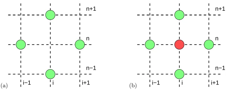
The scheme (99) is distinguished by evaluating the algebraic mass term using the average 12 un
i−1+uni+1
of the points used to approximate the spatial derivativeuxx, rather than introducing the additional pointuni into
the stencil, as shown in figure 6. The scheme (99) thus describes evolution on two interwoven but uncoupled space-time grids connecting the valuesun
i for whichi+nis either always even or always odd.
The discrete scheme (99) is an exact rewriting of the original quantum lattice algorithm (95a,b) forun i and
dn
i. Instead of computing u n+1
i,...,N and d n+1
i,...,N from u n
i,...,N and d n
i,...,N, one stores two time levels u n
i,...,N and
uni,...,N−1 and computesuni,...,N+1 . One may reconstructdni,...,N+1 from uni,...,N+1 andun
i,...,N using (97).
(a)
n+1
n
n−1
i
i−1 i+1 (b)
n+1
n
n−1
i
i−1 i+1
Figure 6. (a) Four point stencil for the three time level algorithm that computesuni+1 from un
i±1andu n−1
i . The algebraic mass term is computed from the average 1 2 u
n
i−1+uni+1
, rather than by enlarging the stencil to include the central pointun
i shown in (b).
the array holding uni,...,N−1 with the newly computed value foruni+1. This reformulation is therefore again much better suited to a multi-threaded parallel implementations, or implementations on GPUs since the calculations of theuni+1overi= 1, . . . , N may be performed in any order. This is in distinct contrast to the requirement for either two sets of arrays or a specialised data layout and streaming algorithm (such as the algorithm by Bailey et al. [71]) for the direct implementation of (95a,b) on a GPU.
11.
Discrete action principle
The complex Klein–Gordon equation (94) may be obtained from the action integral
S= Z
dtL= Z Z
dtdz L= Z Z
dtdz
1 2|ut|
2−1
2|uz|
2−1
2m
2|u|2
(101)
using the complex Hamilton’s principle that variesuand its complex conjugateu? independently [12, 14]
0 = δL δu = ∂ ∂t ∂L ∂ut + ∂ ∂z ∂L ∂uz −∂L ∂u, 0 =
δL δu? =
∂ ∂t ∂L ∂u? t + ∂ ∂z ∂L ∂u? z − ∂L
∂u?. (102)
This is equivalent to writingu=ur+ iui and varying the two real fieldsur and ui independently. The action
integral is the time integral of a Lagrangian functional L, which in turn is the spatial integral of a Lagrangian densityL.
The above three time level scheme (99) is the variational integrator derived from the discrete Hamilton’s principle
∂S ∂un
i
= 0, ∂S ∂un ?
i
= 0, (103)
for the discrete action
S=X
i,n
1 2
uni+1−uni 2
−1 2
uni+1−uni 2
−1 4m˜
2∆t2 un iu
n ? i+1+u
n i
?
uni+1
. (104)
We may identify each of the three terms as discrete approximations to the three terms representing kinetic, elastic, and potential energy in the continuous action (101) using the three points un
i, uni+1, u n+1
i and their
The same discrete action may be rewritten more symmetrically as
S0 =X
i,n 1 2u n i ?
uni−1+uni+1−uni+1−uni−1−1 2m˜
2∆t2 un i−1+u
n i+1
+ complex conjugate. (105)
This form emphasises the symmetry between the grid pointsun
i±1and time levelsu n±1
i in (99). Moreover, this
expression for the action is written asun i
?multiplying the discrete evolution equation forun
i, plusuni multiplying
the discrete evolution equation foruni?, so one may read off the evolution equations directly from the action. The two expressionsS andS0 for the discrete action differ by the telescoping sum
S−S0 =X
i,n
|uni+1|2− |un i+1|
2+1
4m˜
2∆t2 un ? i u
n i−1−u
n ? i+1u
n i +u
n iu
n ? i−1−u
n i+1u
n ? i +1 2 u n ? i u n i+1−u
n ? i−1u
n i +u
n iu
n ? i+1−u
n i−1u
n ? i +u
n ? i u
n−1
i −u
n+1?
i u
n i +u
n iu
n−1?
i −u
n+1 i u n ? i (106)
A telescoping sum is the discrete analogue of a null Lagrangian density L0 for which RRdtdzL0 = 0 in the presence of suitable (e.g. periodic) boundary conditions. For example, the complex Klein–Gordon equation may also be obtained from the continuous action
S0=−1 4
Z Z
dtdz u? utt−uzz+m2u+u u?tt−u ? zz+m
2u?
, (107)
which is related to the previous expressionS in (101) by
S − S0= 1
4 Z Z
dtdz ∂
∂t(u
?u
t+uu?t)−
∂ ∂z(u
?u
z+uu?z)
. (108)
12.
Discrete energy conservation property
The quantum lattice algorithms also satisfy a discrete energy conservation property that complements the above discrete action principle [4]. We write the expectation of a general operator A as hAi =hψ|Aψi for a normalised state withhψ|ψi= 1. This asymmetric notation is required whenAis not Hermitian. The continuous time evolution of an expectation is given by Ehrenfest’s formula [15]
d
dthAi= ih[H,A]i+h∂tAi, (109) where [H,A] =HA−AHis the commutator ofAandH. The h∂tAiterm captures any explicit time-dependence
in A. The Hamiltonian for a closed quantum system cannot depend explicitly on time, so Ehrenfest’s formula establishes that hHiis constant. This expresses the energy conservation property of a closed quantum system evolving in continuous time.
By contrast, the quantum lattice algorithms generate evolution in discrete time steps of length ∆t. We may write |ψn+1i= ˜E|ψni, where|ψni and|ψn+1iare the abstract states at timesnand n+ 1. The discrete
evolution operator ˜E is unitary for a quantum system with no explicit time dependence. Unitary evolution implies conservation of probability,
hψn+1|ψn+1i=hE˜ψn|E˜ψni=hψn|E˜†E˜ψni=hψn|ψni, (110) where the third step ˜E†˜E = 1 uses the unitary property of ˜E. Computing the expectation of the evolution operator itself gives
so the unitary evolution in discrete time steps generated by ˜Econserves the expectation hE˜i=hψ|E˜ψi.
The discrete evolution operator ˜E approximates the formal solution operator E∆t = exp (−i∆tH) for the
evolution of the continuous-time systemi∂tψ=Hψover a timestep ∆t. This evolution conserves the expectation
hE∆ti, sinceE∆t commutes withH. Formally expandinghE∆tifor small ∆tgives
hψ|exp (−i ∆tH)ψi=hψ|ψi −i ∆thψ|Hψi −∆t2hHψ|Hψi+O(∆t3). (112) The leading order termhψ|ψiis the total probability, while the first correction (and the leading order imaginary part) is proportional to the expectation of the Hamiltonian. Conservation of the expectation of the evolution operator E∆t thus encapsulates both conservation of total probability (unitary evolution) and conservation of
energy.
The discrete evolution operator ˜Eis a unitary approximation to E∆t, so the conservation ofh˜Eiunder the
discrete evolution implies conservation of a consistent discrete approximation tohHi. If ˜Eis a first-order in ∆t approximation toE∆t,
i 1 ∆th
˜
E−1i=hHi+O(∆t), (113) and if ˜Eis a second-order approximation,
Re
i 1 ∆th
˜
E−1i
=hHi+O(∆t2). (114)
We now apply these general results to the quantum lattice algorithms for the one-dimensional Dirac equations. Some three-dimensional applications may be found in [4].
12.1.
One-dimensional Dirac equation
The action integral for the Dirac equation may be written in a form analogous to (107) as [12, 14]
SDirac= Z Z
dtdV ψ†
i∂ψ ∂t −Hψ
. (115)
Treating ψ and ψ† as independent variables and varyingψ† gives the Dirac equation in the formi∂tψ=Hψ.
This action may be written in a more symmetric form between ψ and ψ†, analogous to (101), by adding an exact time derivative. The second term in the Lagrangian density is minus the expectation of the Hamiltonian operator,
hHi=hψ|Hψi= Z
dzψ†Hψ, (116)
which is equal to the Hamiltonian functional in classical Lagrangian particle mechanics. For the 1D Dirac equation written in the form (32) the expectation of the Hamiltonian is
hHi= Z
dz
u?(−iuz+ imd−gu) +d?(idz−imu−gd)
. (117)
This is easier to interpret in the variables Φ±= (u±id)/√2,
hHi= Z
dz
m |Φ+|2− |Φ−|2
−g |Φ+|2+|Φ−|2
−i Φ+?∂zΦ−+ Φ−?∂zΦ+
, (118)
as the mass terms for Φ± describe positive and negative energy states. The terms involving spatial derivatives