Malmquist Productivity Index for Multi Time Periods

315

Int. J. Data Envelopment Analysis (ISSN 2345-458X)

Vol.2, No.1, Year 2014 Article ID IJDEA-00213, 8 pages

Research Article

Malmquist Productivity Index for Multi Time

Periods

Y. Jafaria

(a) Department of Mathematics, Shabestar Branch, Islamic Azad University, Shabestar, Iran.

Received 18 July 2013, Revised 11 December 2013, Accepted 6 February 2014

Abstract

The performance of a decision making unit (DMU) can be evaluated in either across-sectional or a time-series manner, and data envelopment analysis (DEA) is a useful method for both types of evaluation. The Malmquist productivity index (MPI) evaluates the change in efficiency of a DMU between two time periods. It is defined as the product of the Catch-up and Frontier-shift terms. In this paper, we study the Malmquist productivity index of a DMU between several time periods.

Keywords: Data envelopment analysis; Malmquist productivity index; Curve fitting.

1. Introduction

Data envelopment analysis (DEA) is a mathematical programming technique, which is used to evaluate the relative efficiency of decision making units (DMUs) and has been proposed by Charnes et al. [1] as the CCR model (the model by Banker et al. [2] usually is referred to as the BCC model). The original idea behind DEA was to provide a methodology whereby, within a set of comparable decision making units (DMUs), those exhibiting best practice could be identified, and would form an efficient frontier. Furthermore, the methodology enables one to measure the level of efficiency of non-frontier units, and to identify benchmarks against which such inefficient units can be compared. Performance measurement is an important issue for at least two reasons. One is that in a group of units where only limited number of candidates can be selected, the performance of each must be evaluated in a fair and consistent manner. The other is that as time progresses, better performance is expected. Hence, the units with declining performance must be identified in order to make the necessary improvements.

In addition to comparing the relative performance of a set of DMUs at a specific period, the conventional DEA can also be used to calculate the productivity change of a DMU over time. Caves et al. [3, 4] have proposed a Malmquist productivity index (MPI) which is calculated the relative

_{Corresponding author: [email protected]}

316 Y.Jafari, et al /IJDEA Vol.2, No.1, (2014).315-322

0 V , 0 U

, n , , 1 j 1 X V

Y U . t . s

X V

Y U Max

j T

j T

o T

o T

 



 

0 V , 0 U

n , , 1 j 0 X V Y U

1 X V . t . s

Y U Max

j T j T

o T

o T

 

 

 



performance of a DMU in different periods of time by using the technology of a base period. Since the base period used to define the production technology affects the results, several modifications for calculating MPI have been proposed. The most popular method is the one proposed by Fare et al. [5] which takes the geometric mean of the MPIs calculated from two base periods. Later, Pastor and Lovell [6] proposed a global MPI, based on a technology defined by DMUs of all periods, to calculate productivity changes. These papers are for using in two time periods. In this paper, we offer using Data Envelopment Analysis for evaluating the performance of Malmquist productivity index for DMUs in several time periods. For evaluating productivity of DMU, We are obtained MPIs in all pairs of consecutive periods. Then by curve fitting, are determined productivity index in several time periods.

The scientific contribution of this paper are: 1) evaluate the performance of DMUs in several time periods. 2) Combining the two indicators, approximate MPIs as the straight line that slope of line is one index and another index is the average MPIs.

The remainder of this paper has the following structure: in section 2, we present the required background. Section 3 introduces our method as a usage of Malmquist productivity index. Section 4 illustrates the proposed method using an example. Finally, conclusions are given in section 5.

2.Background 2.1.DEA Models

Data envelopment analysis (DEA) is a method for evaluating efficiency of decision making units (DMUs). Consider n decision making units DMU_j (j1,,n), each DMUj consuming input levels

) m , , 1 i (

x_ij   to produce output levels y_rj (r1,,s). The relative efficiency score of DMUo under the CCR model is given by the following optimization problem:

(1)

Where U(u1,,us) and V(v1,,vm) represent vectors for the output and input weights, respectively.

We point out that the DEA model (1) is equivalent to the following linear program which is called the input-oriented formulation for the CCR model:

(2)

2.2.Malmquist productivity index

We assume that for each time period t, the production technology t

S is the transformation of inputs, _Xt_{, into outputs, Y}t_{, in other words,} t



t t t t



Y produce can X | ) Y , X (

S  . Now, we the DEA

score for DMUo of the period l measured by means of the period k frontier, we denote it as

) Y , X (

Dk l_{o o}l . Then, we have:

. n , , 1 j , 0 Y Y X X . t . s Min ) Y , X ( D j l o n 1 j k j j l o n 1 j k j j l o l o k           





  (4)

that, k,l{t,t1}.

Malmquist productivity index was illustrated by Caves et. al. [3,4] and listed as follows:

(5)

In this formulation, technology in period is the reference technology. The follow equation represents the productivity of the production point (Xt1,Yt1) relative to the production point

) Y , X

( t t . A value >1 will indicate positive MPI growth from period t to period t1, and vice versa, if that is <1, then MPI have negative growth.

(6)

In the assumption of CRS, the above index can be broken down in to technological change (TECH) and technical efficiency change (EFFCH) indexes and the equation can be written as:

(7) t n , , 1 j , 0 Y Y X X . t . s Min j o n 1 j j j o n 1 j j j          





  ) Y , X ( D ) Y , X ( D M _t o t o t 1 t o 1 t o 1 t t     ) Y , X ( D ) Y , X ( D ) Y , X ( D ) Y , X ( D MPI _t o t o 1 t 1 t o 1 t o 1 t t o t o t 1 t o 1 t o t 1 t , t o        _{ } ) Y , X ( D ) Y , X ( D ) Y , X ( D ) Y , X ( D ) Y , X ( D ) Y , X ( D MI _t o t o 1 t t o t o t 1 t o 1 t o 1 t 1 t o 1 t o t t o t o t 1 t o 1 t o 1 t 1 t , t

o    

      _{  }

318 Y.Jafari, et al /IJDEA Vol.2, No.1, (2014).315-322

MPI measures the productivity change between periods and . Productivity declines if MPI<1, remains unchanged if MPI=1 and improves if MPI>1.

3. Malmquist productivity index for multi time periods

We study performance of a DMU for T time periods. We let X (x , ,xtmj) t

j 1 t

j   and

) y , , y (

Y_jt  ₁t_j _sjt represent input and output vectors for each DMUt_j, (j1,2,,n), (t1,2,,T) of the period . Now, we the DEA score of DMUlo measured by means of the period k frontier, we denote it as and that is determined by problem 4. Then, we can for each two time periods

) T , , 2 , 1 t ( 1 t ,

t    , determine the Malmquist productivity index by using of formula 7.

So, we assume that have all the malmquist productivity index for each DMUj in two time periods

1 t ,

t 

as MPI_ot,t1, (t1,2,,T1).

Now, we consider points of (t,MPIt_o,t1) on the Cartesian coordinates so that the horizontal axis is for time t and the vertical axis is for the malmquist productivity index. Then for DMUo, we have T1 points of (x_t,y_t)(t,MPIt_o,t1) on the Cartesian coordinates.

Now, we can by using of the curve fitting consider Special form of one function and by mathematical methods obtain Function parameters. We want approximate points as one Straight line. So, we consider that function form be as yx that (x,y) are points on coordinate set and , are parameters of function that must be determined. The deviations points (x_t,y_t)(t,MPIt_o,t1) of the straight line is showed as the following:

1 T , , 1 t ), t ( MPI ) x ( y

d_t  _t  _t  _ot,t1     

(8)

that these deviations must be minimized and so for approximation is sufficient that the following problem is solved:

(9)

that  and  are Unknown. To obtain parameters, (9) can be written as a linear problem. Then put:

) 1 T , , 1 t ( 0 v , u , 0 v u , t MPI v

u_t  _t  t_o,t1  _{t t}  _{t t}    

So, the problem 9 is converted to the following problem:

(10)

t t1

t ) Y , X ( Dk l_{o o}l

t t problem as linear programming:

(11)

Now, let in evaluating DMUo the optimal solution is (o,o). Then, the straight line to approximate the performance of this unit in the period T, will be yoxo and we have:

1) If o 0 then DMUo progress has during T periods. 2) If _o 0 then DMUo regression has during T periods. 3) If _o 0 then DMUo has not changed during T periods. Note that certain states such as o  never happens.

Now, suppose we have a DMU that MPI values for that is larger than one and declining. Then method shows that DMU regression has during these periods and so this factor is not enough for evaluate productivity of DMUs. We consider the average MPI values as another factor. Now, the following cases may occur:

1) If method show progress and the average is >1, then DMU is in ideal situation.

2) If method show progress and the average is <1, then DMU isn't currently in good condition but has a good future.

3) If method show regress and the average is >1, then DMU is currently in good condition but has a bad future.

4) If method show regress and the average is <1, then DMU isn't currently in good condition and has a bad future.

4. Numerical example

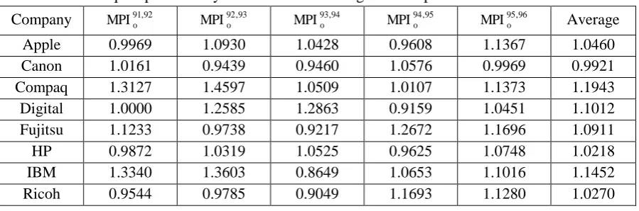
In this section, we present one example of Chen, Ali [7]. In this category, there are eight companies. The calculations are based upon three inputs (i) assets, (ii) shareholder's equity and (iii) the number of employees, and one output, namely, revenue. We first look at the malmquist productivity index. Tables 1 report the DEA the malmquist productivity index from 1991 to 1996.

Table 1.

The malmquist productivity index and their average for companies from 1991 to 1996. Company MPI91o,92

93 , 92 o

MPI MPI93o,94

95 , 94 o

MPI MPI95o,96 Average

Apple 0.9969 1.0930 1.0428 0.9608 1.1367 1.0460

Canon 1.0161 0.9439 0.9460 1.0576 0.9969 0.9921

Compaq 1.3127 1.4597 1.0509 1.0107 1.1373 1.1943

Digital 1.0000 1.2585 1.2863 0.9159 1.0451 1.1012

Fujitsu 1.1233 0.9738 0.9217 1.2672 1.1696 1.0911

HP 0.9872 1.0319 1.0525 0.9625 1.0748 1.0218

IBM 1.3340 1.3603 0.8649 1.0653 1.1016 1.1452

Ricoh 0.9544 0.9785 0.9049 1.1693 1.1280 1.0270

1 T , , 1 t 0

v , u

1 T , , 1 t , t MPI

v u . t . s

) v u ( Min

t t

1 t , t o t

t 1 T

1 t

t t

 



 

    

 

 





320 Y.Jafari, et al /IJDEA Vol.2, No.1, (2014).315-322

Now, we use of section 3 to curve fitting as the straight line. Results of using of model 11 are presented in figure 1.

Figure 1: Result of curve fitting.

Equation of the fitted lines.

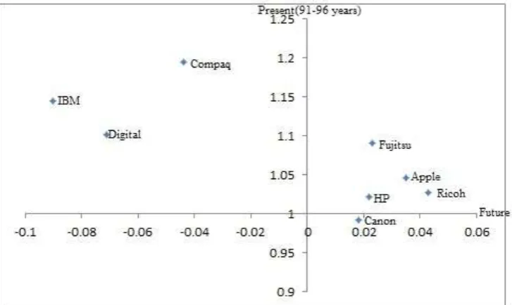
Now, according to tables 1 and 2, we will comment on the performance of companies. For example, Apple is company that progress has during T periods and the average for it is greater than one. So, Apple is in ideal situation and it is currently in good condition and has a good future. In figure 2, results are given for other companies.

Figure 2: Present and future status of companies

It can be seen that the companies (except Canon) between 91 and 96 were making good progress, but growth of IBM, Compaq and Digital show that they have not a good future and the future for Canon is good.

Company Equation Slope() Performance Apple y=0.035x+0.962 0.035 Progress Canon y=0.018x+0.909 0.018 Progress

Compaq

y=-0.044x+1.357 -0.044 Regress

Digital

y=-0.071x+1.401 -0.071 Regress Fujitsu y=0.023x+1.100 0.023 Progress

HP y=0.022x+0.965 0.022 Progress

IBM

322 Y.Jafari, et al /IJDEA Vol.2, No.1, (2014).315-322

5. Conclusions

Malmquist Productivity Index (MPI), based on DEA, is used to measure the performance changes over time. The malmquist Productivity Index allows us to distinguish between shifts in the production frontier (technological change), and movement of departments nearer the frontier (efficiency change). We have prepared a method that by using the malmquist productivity index calculated an index to evaluate the performance of DMUs in several time periods. We approximate MPIs as the straight line that slope of line is one index and another index is the average MPIs.

References

[1]. A. Charnes, W.W. Cooper and E. Rhodes, 1978. Measuring the efficiency of decision making units. European Journal of Operational Research, 2: 429-444.

[2]. R.D. Banker, A. Charnes and W.W. Cooper, 1984. Some models for estimating technical and scale inefficiencies in data envelopment analysis. Management Science, 30(9): 1078-1092.

[3]. D.W. Caves, L.R. Christensen and W.E. Diewert, 1982. The economic theory of index numbers and the measurement of input, output, and productivity. Econometrica, 50: 1393-1414.

[4]. D.W. Caves, L.R. Christensen and W.E. Diewert, 1982. Multilateral comparisons of output, input, and productivity using superlative index numbers. The Economic Journal, 92: 73-86.

[5]. R. Fare, G. rosskopf, M. Norris and Z. Zhang, 1994. Productivity growth, technical progress and efficiency change in industrialized countries. American Economic Review, 84: 66-83.

[6]. J.T. Pastor, C.A.K. Lovell, 2005. A global Malmquist productivity index. Economics Letters, 88: 266-271.