Dynamic Asset Allocation
∗
Claus Munk
†This version: April 4, 2003
∗Informal lecture notes originally prepared for Ph.D. course on Continuous-time Finance, Danish Doctoral
Re-search Programme in Finance, Spring 2001. I appreciate comments and corrections from Heine Jepsen and Nicolai Nielsen.
†Department of Accounting and Finance, University of Southern Denmark, Campusvej 55, DK-5230
Contents
1 Introduction 1
1.1 Investor classes and motives for investments . . . 1
1.2 Typical investment advice . . . 3
1.3 An overview of the theory of optimal investments . . . 3
1.4 The future of investment management and services . . . 3
1.5 Outline of the rest . . . 3
1.6 Notation . . . 3
2 Preferences 4 2.1 Expected utility representation of preferences . . . 4
2.1.1 Basic representation of preferences . . . 4
2.1.2 Expected utility of consumption plans . . . 6
2.1.3 Behavioral axioms and derived properties . . . 6
2.1.4 Expected utility representation of preferences . . . 6
2.1.5 Are the axioms reasonable? . . . 8
2.2 Risk aversion . . . 8
2.2.1 Definitions . . . 8
2.2.2 Comparison of risk aversion between individuals . . . 10
2.3 Frequently applied utility functions . . . 10
2.4 Preferences in multi-period settings . . . 12
3 One-period models 15 3.1 The general one-period model . . . 15
3.2 Mean-variance analysis . . . 16
3.2.1 Theoretical foundation . . . 16
3.2.2 Mean-variance analysis with only risky assets . . . 17
3.2.3 Mean-variance analysis with both risky assets and a riskless asset . . . 19
3.3 Critique of the one-period framework . . . 20
4 Introduction to multi-period models 21 4.1 A multi-period, discrete-time framework . . . 21
4.2 Wealth dynamics . . . 22
4.3 Dynamic programming in discrete-time models . . . 23
4.4 The basic continuous-time setting . . . 25
Contents ii
4.5 Dynamic programming in continuous-time models . . . 28
4.6 The martingale approach to consumption-portfolio problems . . . 32
4.7 Exercises . . . 36
5 Asset allocation with constant investment opportunities 37 5.1 General utility function . . . 37
5.2 CRRA utility function . . . 39
5.3 Logarithmic utility . . . 42
5.4 Discussion of the optimal investment strategy . . . 43
5.5 Exercises . . . 45
6 Asset allocation with stochastic investment opportunities: the general case 47 6.1 One-dimensional state variable . . . 48
6.1.1 General utility functions . . . 48
6.1.2 Specific utility functions . . . 51
6.2 Multi-dimensional state variable . . . 53
6.3 What risks are to be hedged? . . . 55
6.4 Closed-form solution for CRRA utility: affine models with one state variable . . . 56
6.4.1 Utility from terminal wealth only . . . 57
6.4.2 Utility from consumption (and possibly terminal wealth) . . . 59
6.5 Closed-form solution for CRRA utility: quadratic models with one state variable . 61 6.5.1 Utility from terminal wealth only . . . 61
6.5.2 Utility from consumption (and possibly terminal wealth) . . . 63
6.6 Closed-form solution for CRRA utility: multiple state variables . . . 64
6.7 Applying the martingale approach . . . 64
7 Asset allocation with stochastic investment opportunities: concrete cases 67 7.1 Stochastic interest rates . . . 67
7.1.1 One-factor Vasicek interest rate dynamics . . . 68
7.1.2 One-factor CIR dynamics . . . 71
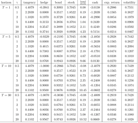
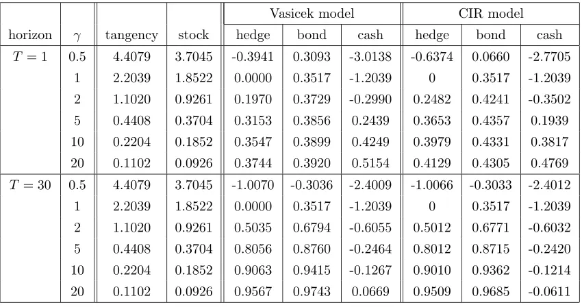
7.1.3 A numerical example . . . 73
7.1.4 Other studies with stochastic interest rates . . . 79
7.2 Stochastic excess returns . . . 79
7.3 Stochastic volatility . . . 82
7.4 Exercises . . . 83
8 Non-financial risks 85 8.1 Labor income . . . 85
8.1.1 Exogenous labor income . . . 85
8.1.2 Endogenous labor supply and income . . . 90
8.1.3 Further references on labor income in portfolio and consumption choice . . 92
8.2 Inflation . . . 92
8.3 Multiple and/or durable consumption goods . . . 96
Contents iii
9 Non-standard assumptions on investors 97
9.1 Preferences with habit formation . . . 97
9.2 Recursive utility . . . 99
9.3 Other objective functions . . . 99
9.4 Consumption and Portfolio Choice for Non-price takers . . . 99
9.5 Non-Utility Based Portfolio Choice . . . 99
9.6 Allowing for Bankruptcy . . . 100
10 Trading and information imperfections 101 10.1 Model/parameter uncertainty or incomplete information . . . 101
10.2 Trading constraints . . . 101
10.3 Transaction Costs . . . 101
11 Computational Methods 102
Chapter 1
Introduction
Financial markets offer opportunities to move money between different points in time and different states of the world. Investors must decide how much to invest in the financial markets and how to allocate that amount between the many, many available financial securities. Investors can change their investments as time passes and they will typically want to do so for example when they obtain new information about the prospective returns on the financial securities. Hence, they must figure out how to manage their portfolio over time. In other words, they must determine a dynamic investment or asset allocation strategy. The term asset allocation is sometimes used for the allocation of investments to major asset classes, e.g. stocks, bonds, and cash. In later chapters we will often focus on this decision, but we will use the term asset allocation interchangeably with the terms optimal investment or portfolio management.
It is intuitively clear that in order to determine the optimal investment strategy for an investor, we must make some assumptions about the objectives of the investor and about the possible returns on the financial markets. Different investors will have different motives for investments and hence different objectives. In Section 1.1 we will discuss the motives and objectives of different types of investors. We will focus on the asset allocation decisions of individual investors or households. Individuals invest in the financial markets to finance future consumption of which they obtain some felicity or utility. We discuss how to model the preferences of individuals in Chapter 2.
1.1
Investor classes and motives for investments
We can split the investors into individual investors (households; sometimes called retail in-vestors) and institutional investors (includes both financial intermediaries – such as pension funds, insurance companies, mutual funds, and commercial banks – and manufacturing companies pro-ducing goods or services). Different investors have different objectives. Manufacturing companies probably invest mostly in short-term bonds and deposits in order to their liquidity needs and avoid the deadweight costs of raising small amounts of capital very frequently. They will rarely set up long-term strategies for investments in the financial markets and their financial investments is a very small part of the total investments.
Individuals can use their money either for consumption or savings. Here we use the term savings synonymously with financial investments so that it includes both deposits in banks and investments in stocks, bonds, and possibly other securities. Traditionally most individuals have saved in form of bank deposits and maybe government bonds, but in recent years there has been
1.1 Investor classes and motives for investments 2
an increasing interest of individuals for investing in the stock market. Individuals typically save when they are young by consuming less than the labor income they earn, primarily in order to accumulate wealth they can use for consumption when they retire. Other motives for saving is to be able to finance large future expenditures (e.g. purchase of real estate, support of children during their education, expensive celebrations or vacations) or simply to build up a buffer for “hard times” due to unemployment, disability, etc. The objective of an individual investor is to maximize the utility of consumption throughout the life-time of the investor. We will discuss utility functions in Chapter 2.
A large part of the savings of individuals are indirect through pension funds and mutual funds. These funds are the major investors in today’s markets. Some of these funds are non-profit funds that are owned by the investors in the fund. The objective of such funds should represent the objectives of the fund investors.
Let us look at pension funds. One could imagine a pension fund that determines the optimal portfolio of each of the fund investors and aggregates over all investors to find the portfolio of the fund. Each fund investor is then allocated the returns on his optimal portfolio, probably net of some servicing fee. The purpose of the fund is then simply to save transaction costs. A practical implementation of this is to let each investor allocate his funds among some pre-selected portfolios, for example a portfolio mimicking the overall stock market index, various portfolios of stock in different industries, one or more portfolios of government bonds (e.g. one in short-term and one in long-term bonds), portfolios of corporate bonds and mortgage-backed bonds, portfolios of foreign stocks and bonds, and maybe also portfolios of derivative securities and even non-financial portfolios of metals and real estate. Some pension funds operate in this way and there seems to be a tendency for more and more pension funds to allow investor discretion with regards to the way the deposits are invested.
However, in many pension funds some hired fund managers decide on the investment strategy. Often all the deposits of different fund members are pooled together and then invested according to a portfolio chosen by the fund managers (probably following some general guidelines set up by the board of the fund). Once in a while the rate of return of the portfolio is determined and the deposit of each investor is increased according to this rate of return less some servicing fee. In many cases the returns on the portfolio of the fund are distributed to the fund members using more complicated schemes. Rate of return guarantees, bonus accounts,.... The salary of the manager of a fund is often linked to the return on the portfolio he chooses and some benchmark portfolio(s). A rational manager will choose a portfolio that maximizes his utility and that portfolio choice may be far from the optimal portfolio of the fund members....
Mutual funds...
This lecture note will focus on the decision problem of an individual investor and aims to analyze and answer the following questions:
• What are the utility maximizing dynamic consumption and investment strategies of an indi-vidual?
• What is the relation between optimal consumption and optimal investment?
1.2 Typical investment advice 3
• How are financial investments optimally allocated to single securities within each asset class? • How does the optimal consumption and investment strategies depend on, e.g., risk aversion,
time horizon, initial wealth, income, and asset price dynamics?
• Are the recommendations of investment advisors consistent with the theory of optimal in-vestments?
1.2
Typical investment advice
1.3
An overview of the theory of optimal investments
1.4
The future of investment management and services
See Bodie (2003), Merton (2003)
1.5
Outline of the rest
1.6
Notation
Since we are going to deal simultaneously with many financial assets, it will often be mathe-matically convenient to use vectors and matrices. All vectors are considered column vectors. The superscript > on a vector or a matrix indicates that the vector or matrix is transposed. We will
use the notation1for a vector where all elements are equal to 1 – the dimension of the vector will be clear from the context. We will use the notationeifor a vector (0, . . . ,0,1,0, . . . ,0)>where the 1 is entry number i. Note that for two vectorsx= (x1, . . . , xd)> and y = (y1, . . . , yd)> we have
x>y=Pd
i=1xiyi. Also,x>1=
Pd
i=1xi ande>i x=xi.
If x= (x1, . . . , xn) and f is a real-valued function of x, then the (first-order) derivative off
with respect toxis the vector
f0(x) =
∂ f ∂x1
, . . . , ∂ f ∂xn
>
.
This is also called the gradient off. The second-order derivative off is then×nHessian matrix
f00(x) =
∂2f
∂x2 1
∂2f
∂x1∂x2 . . .
∂2f
∂x1∂xn ∂2f
∂x2∂x1
∂2f
∂x2 2 . . .
∂2f
∂x2∂xn ..
. ... . .. ... ∂2f
∂xn∂x1
∂2f
∂xn∂x2 . . .
∂2f
∂x2
n
.
Ifxandaare n-dimensional vectors, then
∂ ∂x(a
>x) =a.
Ifxis an n-dimensional vector and Ais a symmetric [i.e.A=A>] n×nmatrix, then
∂ ∂x(x
Chapter 2
Preferences
There is a large literature on how to model the preferences of individuals for uncertain outcomes. The literature dates back at least to Daniel Bernoulli in 1738 (see English translation in Bernoulli (1954)), but was put on a firm formal setting by von Neumann and Morgenstern (1944). Some recent textbook presentations are given by Huang and Litzenberger (1988, Ch. 1) and Kreps (1990, Ch. 3). The short presentation below mainly follows that of Huang and Litzenberger.
2.1
Expected utility representation of preferences
2.1.1 Basic representation of preferences
• Assume a single consumption good and a one-period economy with uncertainty about the state ω ∈ Ω at time 1 (end-of-period). The probabilities of the states of nature are given [objective].
• A consumption plan x is a specification of the number of units consumed in each state,
x= (xω|ω∈Ω). The set of possible consumption plans is denotedX.
• Assume there are finitely many possible consumption levels, i.e. a finite setZ ⊆Rexist such that xω∈Z for allω∈Ω and allx∈X.
• A preference relationonPis a binary relation satisfying
(i) pqandqr⇒pr [transitivity] (ii) ∀p, q∈P:pqorqp[completeness] • Derived relations∼,6, and...
• A probability distribution on Z is a functionp:Z →[0,1] such thatp(z)≥0,∀z ∈Z and
P
z∈Zp(z) = 1.
• Assume that the preferences of an individual can represented by a preference relation on the set P ≡ P(Z) of probability distributions (aka. lotteries) defined on Z. [...state-independence]
• A utility functionis a functionU:P→Rsuch that
pq⇔U(p)≥U(q).
2.1 Expected utility representation of preferences 5
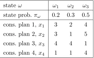
stateω ω1 ω2 ω3
state prob.πω 0.2 0.3 0.5 cons. plan 1,x1 3 2 4
cons. plan 2,x2 3 1 5
cons. plan 3,x3 4 4 1
cons. plan 4,x4 1 1 4
Table 2.1: The possible state-contingent consumption plans in the example.
cons. levelz 1 2 3 4 5
cons. plan 1,p1 0 0.3 0.2 0.5 0
cons. plan 2,p2 0.3 0 0.2 0 0.5
cons. plan 3,p3 0.5 0 0 0.5 0
[image:9.595.208.363.97.193.2]cons. plan 4,p4 0.5 0 0 0.5 0
Table 2.2: The probability distributions corresponding to the state-contingent consumption plans shown in Table 2.1. .
A preference relation can always be represented by a utility function (also ifPis infinite). A utility function is unique up to a strictly positive transformation.
• A von Neumann-Morgenstern utility functionis a functionu:Z→Rsuch that
pq⇔X
z∈Z
p(z)u(z)
| {z }
E[u(˜zp)]
≥X z∈Z
q(z)u(z)
| {z }
E[u(˜zq)]
.
Given a von Neumann-Morgenstern utility function u, a utility function U is defined by
U(p) = E[u(˜zp)].
Example 2.1Consider an economy with three possible states and four possible state-contingent
consumption plans as illustrated in Table 2.1. Note that Z = {1,2,3,4,5}. The probability distributions corresponding to these consumption plans are then as shown in Table 2.2. Note that
2.1 Expected utility representation of preferences 6
2.1.2 Expected utility of consumption plans
Expected utility of consumption planxcorresponding to a probability distributionp:
E[u(x)] =X ω∈Ω
πωu(xω)
=X
z∈Z
X
ω:xω=z
πωu(xω)
=X
z∈Z
u(z) X ω:xω=z
πω
=X
z∈Z
u(z)p(z).
2.1.3 Behavioral axioms and derived properties
Axiom 2.1 is a preference relation.
Axiom 2.2 (Substitution/independence) For allp, q, r∈Pand all a∈(0,1]:
pq⇒ap+ (1−a)raq+ (1−a)r.
Axiom 2.3 (Archimedean) For all p, q, r∈Pwith pqr there exist constantsa, b∈(0,1)
such that
ap+ (1−a)rqbp+ (1−b)r.
From these basic axioms the following properties can be derived:
Theorem 2.1 (1) pq and0≤a < b≤1 ⇒bp+ (1−b)qap+ (1−a)q.
(2) pqrandpr⇒ ∃!a∗∈[0,1] :q∼a∗p+ (1−a∗)r.
(3) pq,rs, anda∈[0,1]⇒ ap+ (1−a)raq+ (1−a)s. (4) p∼qanda∈[0,1]⇒p∼ap+ (1−a)q.
(5) p∼qanda∈[0,1]⇒ap+ (1−a)r∼aq+ (1−a)r for allr∈P. (6) ∃z0, z
0∈Z such that Pz0 pPz0 for allp∈P.
2.1.4 Expected utility representation of preferences
Theorem 2.2 Assume Z finite. A binary relationhas an expected utility representation if and
only ifsatisfies Axioms 1-3.
Proof: First we prove the implication ‘⇐’: Letz0, z
0be as in Property 6. IfPz0∼Pz0 thenp∼q
for allp, q∈Pand consequently anyu(z) =k,∀z∈Z, will do.
Assume now Pz0 Pz0. By Property 2, there exists for any pa unique ap ∈[0,1] such that apPz0+ (1−ap)Pz0 ∼p. Define the functionU :X →RbyU(p) =ap. Then
2.1 Expected utility representation of preferences 7
U is linear:
ap+ (1−a)q∼a[U(p)Pz0+ (1−U(p))Pz0] + (1−a) [U(q)Pz0+ (1−U(q))Pz0]
∼[aU(p) + (1−a)U(q)]Pz0+ [a(1−U(p)) + (1−a)(1−U(q))]Pz0,
henceU(ap+ (1−a)q) =aU(p) + (1−a)U(q). Defineu:Z→Rbyu(z) =U(Pz). Then
U(p) =U X
z∈Z
p(z)Pz
!
=X
z∈Z
p(z)U(Pz) =X z∈Z
p(z)u(z).
Next we prove the implication ‘⇒’: Axiom 1 is simple. Axiom 2: if Pz∈Zp(z)u(z) > P
z∈Zq(z)u(z) then
X
z∈Z
(ap(z) + (1−a)r(z))u(z)>X
z∈Z
(aq(z) + (1−a)r(z))u(z).
Axiom 3: SupposePzp(z)u(z)>Pzq(z)u(z)>Pzr(z)u(z). Define
a= 1−1 2
P
zp(z)u(z)−
P
zq(z)u(z)
P
zp(z)u(z)−
P
zr(z)u(z)
∈(0,1).
Then
X
z
(ap(z) + (1−a)r(z))u(z) =X z
p(z)u(z) + (1−a) X z
r(z)u(z)−X z
p(z)u(z)
!
=X
z
p(z)u(z)−12 X z
p(z)u(z)−X z
q(z)u(z)
!
=1 2
X
z
p(z)u(z) +X z
q(z)u(z)
!
>X
z
q(z)u(z).
Similarly forb. 2
Theorem 2.3 A von Neumann-Morgenstern utility function for a given preference relation is only
determined up to a strictly positive affine transformation, i.e. if uis von Neumann-Morgenstern utility function for, then v will be so if and only if there exist constants a >0 and b such that
v(z) =au(z) +b for allz∈Z.
SupposeUis a utility function with an associated von Neumann-Morgenstern utility function
u. Iff is any strictly increasing transformation, then V =f◦Uis also a utility function for the same preferences, but f ◦uis only the von Neumann-Morgenstern utility function for V if f is affine.
Infinite Z. What ifZ is infinite, e.g.Z=R+≡[0,∞)? It can be shown that...
A preference relation satisfies Axioms 1-3 + an Axiom 4 + “some technical conditions” ⇔ has an expected utility representation.
2.2 Risk aversion 8
Boundedness of expected utility. Suppose uis unbounded from above and R+ ⊆Z. Then
there exists (zn)∞
n=1 ⊆Z with zn → ∞and u(zn)≥2n. Expected utility of consumption plan p withp(zn) = 1/2n:
∞ X
n=1
u(zn)p(zn)≥
∞ X
n=1
2n 1 2n =∞.
If q, r are such that p q r, then the expected utility of q and r must be finite. But for no
b∈(0,1) do we have
qbp+ (1−b)r [expected utility =∞].
• no problem ifZ is finite
• no problem ifR+⊆Z,uis concave, and consumption plans have finite expectations:
uconcave⇒uis differentiable in some point band
u(z)≤u(b) +u0(b)(z−b), ∀z∈Z.
Ifx∈X has finite expectations, then
E[u(x)]≤E[u(b) +u0(b)(x−b)] =u(b) +u0(b) (E[x]−b)<∞.
2.1.5 Are the axioms reasonable?
Let us consider an example illustrating the so-called Allais Paradox. Suppose Z ={0,1,5}. Consider consumption plans
p1= (0,1,0) p2= (0.01,0.89,0.1) p3= (0.9,0,0.1) p4= (0.89,0.11,0).
Theory says: p1p2⇒p4p3. Proof:
0.11($1) + 0.89 ($ 1) ∼p1p2∼0.11
1
11($0) + 10 11($5)
+ 0.89 ($1) ⇒
0.11($1) + 0.89 ($ 0)
| {z }
p4∼
0.11
1 11($0) +
10 11($5)
+ 0.89 ($0) ∼0.9($0) + 0.1($5)
| {z }
p3∼
But: people preferringp1top2often choosep3overp4. People tend to over-weight small probability
events, e.g. ($0) inp2.
Other “problems”:
• the “framing” of possible choices seem to affect decisions • models assume individuals have unlimited rationality But... Still useful! No clear alternatives!
2.2
Risk aversion
2.2.1 Definitions
An individual is said to be risk averse if he prefers the expected value of a lottery to the lottery, i.e. for any consumption plan xwith associated probability functionp, PE[x] p. A risk
2.2 Risk aversion 9
Theorem 2.4 An individual with a von Neumann-Morgenstern utility function u is risk averse
⇔uis concave.
We will focus on greedy and risk averse investors so that the von Neumann-Morgenstern utility functionsuwe shall apply haveu0>0 and u00<0.
Consider a gamble (h1, h2) with probabilities (¯p,1−p¯) such that ¯ph1+ (1−p¯)h2 = 0. For a
risk averse individual we have
u(¯p(z+h1) + (1−p¯)(z+h2)) =u(z)≥pu¯ (z+h1) + (1−p¯)u(z+h2),
i.e.uis concave. And conversely. Similarly: Risk lover, risk neutral...
Thecertainty equivalent of a consumption planpis defined as thez∗∈Z such that
u(z∗) =X
z∈Z
u(z)p(z).
ForZ⊆R,z∗uniquely exists if uis continuous and strictly increasing.
For a risk averse individual we havez∗<P
z∈Zzp(z). The risk compensation that a risk averse individual demands in order to participate in the lotteryz is equal toPz∈Zzp(z)−z∗.
The degree of risk aversion is associated with u00, but good measure should be invariant to
strictly positive, affine transformations. This is satisfied by the Arrow-Pratt measures of risk aversion defined as follows. The Absolute Risk Aversionis given by ARA(z) =−uu000((zz)). The
Relative Risk Aversionis given by RRA(z) =−zuu000((zz)) =zARA(z).
Consider a mean-zero gamble haroundz. Then
E[u(z+h)] =u(z∗) =u(z−π(z, h)).
We can approximate the left-hand side by
E[u(z+h)]≈E
u(z) +hu0(z) +1
2h
2u00(z)
=u(z) +1
2Var[h]u
00(z)
and the right-hand side by
u(z−π(z, h))≈u(z)−π(z, h)u0(z).
Hence we can write the risk compensation as
π(z, h)≈ −1 2Var[h]
u00(z) u0(z) =
1
2Var[h] ARA(z). Of course, the approximation is more accurate for “small” gambles.
We see that the absolute risk aversion ARA(z) is constant if and only ifπ(z, h) is independent ofz.
Probably π(z, h) is decreasing in z, which implies decreasing absolute risk aversion (DARA utility). Note that
ARA0(z) =−u
000(z)u0(z)−u00(z)2
u0(z)2 =
u00(z) u0(z)
2
−u
000(z)
u0(z) <0 ⇒ u
000(z)>0,
2.3 Frequently applied utility functions 10
The Arrow-Pratt risk aversion measures are not changed by increasing, affine transformations ofU.
Loosely speaking, the absolute risk aversion ARAU(W) measures the aversion to a fair gamble of a given dollar amount, such as a gamble where there is an equal probability of winning or loosing 1000 dollars. Since we expect that a wealthy investor will be less averse to that gamble than a poor investor, the absolute risk aversion is expected to be a decreasing function of wealth. The relative risk aversion RRAU(W) measures the aversion to a fair gamble of a given percentage of wealth, such as a gamble where there is an equal probability of winning or loosing 0.05W. Note that utility functions with constant or decreasing (or even modestly increasing) relative risk aversion will display decreasing absolute risk aversion.
2.2.2 Comparison of risk aversion between individuals
An individual with von Neumann-Morgenstern utility functionuis said to be more risk averse than an individual with von Neumann-Morgenstern utility functionv, if for any lotteryp∈Pand ¯
z∈Z withPz∈Zp(z)u(z)≥u(¯z), we havePz∈Zp(z)v(z)≥v(¯z).
Theorem 2.5 u is more risk averse than v ⇔ ARAu(z)≥ ARAv(z), ∀z ∈Z ⇔ there exists f
strictly increasing and concave such thatu=f ◦v.
2.3
Frequently applied utility functions
Let us look at some concrete von Neumann-Morgenstern utility functions that are frequently applied:
CRRA utility. (Also known as power utility, isoelastic utility.) Utility functionsu(W) in this
class are defined forW ≥0:
u(W) =W
1−γ
1−γ, (2.1)
whereγ >0. Note that
ARAu(W) = γ
W, RRAu(W) =γ.
The relative risk aversion is constant across wealth levels, hence the name CRRA (Constant Relative Risk Aversion) utility. Furthermore, u0(0+) ≡ limW
→0u0(W) = ∞ and u0(∞) ≡
limW→∞u0(W) = 0. Some authors assume a utility function of the form u(W) =W1−γ, which
only makes sense for γ ∈ (0,1). However, empirical studies indicate that most investors have a relative risk aversion above 1.
Except for a constant, the utility function
u(W) = W
1−γ−1 1−γ
is equal to the utility function specified in (2.1). The two utility functions are therefore equivalent in the sense that they generate the same optimal choices. The advantage in using the latter definition is that this function has a well-defined limit asγ →1. From l’Hˆospital’s rule we have that
lim γ→1
W1−γ−1 1−γ = limγ→1
−W1−γlnW
2.3 Frequently applied utility functions 11
which is the important special case of logarithmic utility. When we consider CRRA utility, we will assume the simpler version (2.1), but we will use the fact that we can obtain the optimal strategies of a log-utility investor as the limit of the optimal strategies of the general CRRA investor asγ→1.
HARA utility. (Also known as extended power utility.) Utility functions in this class are of the
form
u(W) = γ 1−γ
aW
γ +η 1−γ
(2.2)
with
γ6= 0, a >0, aW
γ +η >0, andη= 1 ifγ=∞.
In this case
ARAu(W) = W 1 γ +
η a
, RRAu(W) = WW γ +
η a
.
The absolute risk aversion is a hyperbolic function of W, hence the name HARA (Hyperbolic Absolute Risk Aversion) utility. Clearly, when η = 0 and γ > 0 we are back to CRRA utility. Therefore, CRRA utility functions belong to the HARA utility function class.
Applying the fact that increasing affine transformations do not change decisions, HARA utility functions can be divided into three different subclasses:
• u(W) = (W−1W−¯γ)1−γ with γ > 0. The limit as γ → 1 of the equivalent utility function
(W−W¯)1−γ−1
1−γ is equal to the extended log utility function u(W) = ln(W −W¯). Utility is defined for W ≥ W¯ and u0( ¯W) = ∞, hence ¯W is often referred to as a subsistence level
of wealth/consumption. This makes sense only if ¯W ≥0. We will refer to this subclass as
subsistence HARA utility functions. For ¯W = 0 we recover the CRRA utility.
• u(W) =−( ¯W−W)1−γ withγ <0. Utility is defined forW ≤W¯, so that we can think of ¯
W as a satiation level. We could call this subclasssatiation HARA utility functions.
• u(W) = −e−aW corresponding to the limit of (2.2) as γ → ∞ and η = 1. This is the
(negative) exponential utility which displays constant absolute risk aversion (CARA) –
not very reasonable!
Since it is hard to imagine negative consumption, most attention has been given to the CRRA utility functions and (to a smaller extent) the non-CRRA subsistence HARA utility functions. There is also a technical advantage to subsistence HARA and to CRRA functions: Sinceu0( ¯W+) =
∞, an optimal solution will have the property that consumption/wealthW will be strictly above ¯W
with probability one. For example, with CRRA utility, we can ignore a non-negativity constraint on consumption since the constraint will never be binding. For computational purposes the negative exponential utility function is often used in connection with normally distributed returns, e.g. in one-period models as discussed below.
2.4 Preferences in multi-period settings 12
2.4
Preferences in multi-period settings
Above we implicitly considered preferences for consumption at one given future point in time. However, we can generalize the ideas and results to multi-period settings. Consider first a discrete time set{0,1,2, . . . , T}. Then the appropriate consumption space isZ ={(z0, z1, z2, . . . , zT)}and consumption plans are represented by a probabilityponZ.
Again, for finiteZ, we have that for a preference relationsatisfying the Axioms 2.1–2.3 there exists a functionU :Z →Rsuch that
pq⇔X
z∈Z
U(z0, z1, . . . , zT)p(z= (z0, z1, . . . , zT)) ≥X
z∈Z
U(z0, z1, . . . , zT)q(z= (z0, z1, . . . , zT)), i.e. the consumption plans are ordered by expected utility. We can call U a multi-period von Neumann-Morgenstern utility function. Note that it depends on consumption at all dates. Again this result can be extended to the case of an infiniteZ, e.g.Z=RT++1, but also to continuous-time settings whereU will then be a function of the entire consumption processc= (ct)t∈[0,T].
In multi-period settings it is important to know to which degree the investor is willing to shift consumption from one point in time to another. A measure of this is given by theintertemporal
elasticity of substitution. The intertemporal elasticity of substitution between consumption at
timetand times(withs > t) is defined as
IESU(ct, cs) =− ∂ U ∂cs
∂ U
∂ct
cs/ct
d(cs/ct)
d∂ U∂c
s
∂ U ∂ct
. (2.3)
Oftentime-additivity is assumed so that the utility the agent gets from consumption in one period does not directly depend on what she consumed in earlier periods or what she plan to consume in later periods. For the discrete-time case, this means that
U(c0, c1, . . . , cT) = T
X
t=0
ut(ct)
where each ut qualifies as a von Neumann-Morgenstern utility function in a one-period setting. Still, when the agent has to choose her current consumption rate, she will take her prospects for future consumption into account. As we shall see, she will in fact try to smooth her consumption rates across time. We will sometimes allow for a utility from leaving wealth for bequest. Letting
WT denote the wealth level after consumption at timeT and ¯uthe bequest utility function, the life-time utility is then given by
U(c0, c1, . . . , cT, WT) = T
X
t=0
ut(ct) + ¯u(WT)
The continuous time analogue is
U(c, WT) =
Z T
0
ut(ct)dt+ ¯u(WT).
2.4 Preferences in multi-period settings 13
the agent prefers to consume any given number of goods sooner than later. This is modeled by the subjective time preference rateδ, which we assume to be constant over time and independent of the consumption level. For a unified notation we replace ¯u(WT) by e−δTu¯(WT). In sum, the life-time utility is typically assumed to be given by
U(c0, c1, . . . , cT, WT) = T
X
t=0
e−δtu(ct) +e−δTu¯(WT)
in discrete-time models and
U(c, WT) =
Z T
0
e−δtu(ct)dt+e−δTu¯(W T) in continuous-time models.
These assumptions on preferences will simplify many computations and facilitate analytical solutions to optimal investment and consumption problems. However, it is important to realize that the time-additive specification does not follow from the basic axioms of choice under uncertainty, but is in fact a strong assumption, which most economists agree is not very realistic. For a time-additive utility specification the intertemporal elasticity of substitution becomes
IESu(ct, cs) =−u
0(cs)/u0(c
t
cs/ct
d(cs/ct)
d(u0(cs)/u0(ct)). (2.4)
When we lets→t, we obtain the instantaneous elasticity of substitution at timet: IESu(ct) =− u
0(ct)
u00(ct)ct. (2.5)
Note that this is equal to the inverse of the relative risk aversion, i.e.
IESu(ct) = 1
RRAu(ct). (2.6)
This result is due to the assumption of time-additive utility. For the special case of power utility, we have RRAu(c) =γ and hence IESu(c) = 1/γ.
The close link between IES and RRA is restrictive. IES and RRA measure two different aspects of preferences. The IES measures the willingness of the individual to substitute consumption over time, whereas the RRA measures the reluctance to substitute consumption across different states of the economy. There is nothing in the theory of choice under uncertainty that links these two concepts together. It is an unfortunate consequence of the assumption of time-additive utility.
According to Browning (1991), non-additive preferences were already discussed in the 1890 book “Principles of Economics” by Alfred Marshall. See Browning’s paper for further references to the critique on intertemporally separable preferences. A relatively simple and therefore also quite tractable example of non-additive preferences is obtained by letting the utility associated with the choice of consumption at a given date may depend on past choices of consumption. This is modeled by replacing u(ct) by u(ct, ht), whereuis decreasing inht, which is a measure of the standard of living or the habit level of consumption, e.g. a weighted average of past consumption rates:
ht=h0e−βt+α
Z t
0
e−β(t−s)c
sds,
whereh0,α, andβ are non-negative constants. High past consumption generates a desire for high
2.4 Preferences in multi-period settings 14
to as preferences withhabit formation. In particular, models whereu(ct, ht) is assumed to be of the power-linear form,
u(c, h) = 1
1−γ(c−h)
1−γ, γ >0, c ≥h,
turn out to be computationally tractable. See Section 9.1 on portfolio and consumption choice for investors with power-linear habit formation preferences.
Another non-additive model of preference is given by the so-called recursive preferences, sug-gested and discussed by, e.g., Kreps and Porteus (1978), Epstein and Zin (1989, 1991), and Weil (1989). The original motivation of this representation of preferences is that it allows individuals to have preferences for the timing of resolution of uncertainty, which is not the case with standard multi-period von Neumann-Morgenstern preferences. With recursive preferences the felicityUt at some point in timetdepends both on consumption and that date and expectations of next period’s felicity. The most tractable, non-trivial specification is
Ut=
(1−δ)c(1t−γ)/θ+δ
EthUt1+1−γi1/θ
θ/(1−γ)
, θ≡ 1−γ 1− 1
ψ
. (2.7)
Hereγhas the interpretation of the relative risk aversion andψthe interpretation of the intertem-poral elasticity of substitution. When γ = 1/ψ, we have θ = 1, and it can be shown that the recursive equation above is satisfied by the standard time-additive power utility. The continuous-time equivalent of recursive utility is called stochastic differential utility and studied by, e.g., Duffie and Epstein (1992).
Chapter 3
One-period models
3.1
The general one-period model
Given d risky assets with (stochastic) rates of return R = (R1, . . . , Rd)> and a riskfree asset
with a (certain) rate of return r over the period of interest. An investor with initial wealthW0
who invests amountsθ= (θ1, . . . , θd)> in the risky assets and the remainderθ0=W0−θ>1in the
riskfree asset will end up with wealth
W =W0+θ>R+θ0r= (1 +r)w0+θ>(R−r1)
at the end of the period. Letting πi =θi/W0 denote the fraction of wealth invested in the i’th
asset, we can rewrite the terminal wealth as
W =W0[1 +r+π>(R−r1)],
whereπ= (π1, . . . , πd)>. The one-period utility-maximization problem is to chooseπto maximize
E[u(W)]. Note that we ignore any consumption decision at the beginning of the planning period, i.e. we assume that the consumption decision has already been taken independently of the investment decision.
Without further assumptions one can show a number of interesting results on the optimal portfolio choice. We will state only a few and refer to Merton (1992, Ch. 2) for further properties of the general solution to this utility maximization problem.
Theorem 3.1 An individual with strictly increasing and concave u will avoid any positive risky
investment only ifE[Rj]≤rfor allj.
Theorem 3.2 Assume a single risky asset. The optimal risky investment θ = θ(W0) has the
following properties:
(i) ifARA(·)is uniformly decreasing/increasing/constant, thenθis increasing/decreasing/constant in W0
(ii) ifRRA(·)is uniformly decreasing/increasing/constant, thenθ/W0is increasing/decreasing/constant
in W0.
3.2 Mean-variance analysis 16
3.2
Mean-variance analysis
Mean-variance analysis was introduced by Markowitz (1952, 1959). Our presentation is inspired by Huang and Litzenberger (1988, Ch. 3). Mean-variance analysis assumes that the portfolio choice of investors will depend only on the mean and variance of their end-of-period wealth and hence on the mean and variances of the portfolios investors can form. Before we go into the derivations of optimal portfolios, let us discuss the theoretical foundation of mean-variance analysis.
3.2.1 Theoretical foundation
In general an individual’s utility of wealth will depend on all moments of wealth. This can be seen by the Taylor expansion ofu(W) around the expected wealth, E[W]:
u(W) =u(E[W]) +u0(E[W])(W−E[W]) +1
2u
00(E[W])(W−E)2+
∞ X
n=3
1
n!u
(n)(E[W])(W
−E[W])n,
whereu(n)is then’th derivative ofu. Taking expectations, we get
E[u(W)] =u(E[W]) +1 2u
00(E[W]) Var(W) + ∞ X
n=3
1
n!u
(n)(E[W]) E [(W
−E[W])n].
A greedy and risk averse investor clearly prefers higher expected wealth and lower variance of wealth, other things equal, but the expected utility is also influenced by higher order moments. Of course, with quadratic utility, the derivatives ofuof order 3 and higher are zero, so the higher order moments of wealth are irrelevant. However, quadratic utility is a very unrealistic model of investor preferences.
Mean-variance analysis is valid if the returns on the risky assets are multivariate normally distributed,R∼N(µ,Σ), then the well-known mean-variance analysis applies. Here,µis a vector of the expected rates of return on the risky assets, and Σ is the variance-covariance matrix of these rates of return, so that Σijdenotes the covariance between the returns on assetiand assetj. Given that the returns on all individual assets are normally distributed, the return on any portfolio – being a weighted average of the returns on the assets in the portfolio – will also be normally distributed. A portfolio characterized by the portfolio weightsπhas a return ofRπ ≡π>R=Pd
i=1πiRi, which is normally distributed with mean and variance given by
µ(π)≡E[Rπ] =π>µ=
d
X
i=1
πiµi, (3.1)
σ2(π)≡Var[Rπ] =π>Σπ=
d
X
i=1
d
X
j=1
πiπjΣij. (3.2)
Consequently, the end-of-period wealth of each investor will also be normally distributed for any portfolio choice. All higher-order moments of wealth can be written in terms of mean and variance so that expected utility depends only on expected wealth and the variance of wealth.
3.2 Mean-variance analysis 17
individual assets are lognormally distributed, ruling out negative prices and rates of return below 100%. The lognormal distribution is also fully described by its first two moments. Unfortunately, such an assumption is not tractable in a one-period setting since neither the value nor the return on a portfolio will then not be lognormally distributed (the lognormal distribution is not stable under addition).
3.2.2 Mean-variance analysis with only risky assets
Assume that the variance-covariance matrix Σ is non-singular, which is the case if none of the assets are redundant, i.e. no asset has a return which is linear combination of the returns of other assets. The inverse of Σ is denoted by Σ−1. A portfolio is said to bemean-variance efficient if
it has the minimum return variance among all the portfolios with the same mean return. Given the normality assumption on returns, greedy and risk averse investors will only choose among the mean-variance portfolios. Assuming that there are no portfolio constraints, we can find a mean-variance portfolio with expected return ¯µby solving the quadratic minimization problem
min π
1 2π
>Σπ
s.t. π>µ= ¯µ,
π>1= 1.
(3.3)
The ‘12’ in the objective will be notationally convenient when we solve the problem. Clearly, the portfolio that minimizes half the variance will also minimize the variance.
We solve the problem by the Lagrange technique. Letting αandβ denote the Lagrange mul-tipliers of the two constraints, the Lagrangian is
L= 1 2π
>Σπ+α(¯µ−π>µ) +β(1−π>1).
The first-order condition with respect toπ is
∂L
∂π = Σπ−αµ−β1= 0,
which implies that
π=αΣ−1µ+βΣ−11. (3.4)
The first-order conditions with respect to the multipliers simply give the two constraints to the minimization problem. Substituting the expression (3.4) forπinto the two constraints, we obtain the equations
αµ>Σ−1µ+β1>Σ−1µ= ¯µ,
αµ>Σ−11+β1>Σ−11= 1.
Defining
A=µ>Σ−1µ, B=µ>Σ−11=1>Σ−1µ, C=1>Σ−11,
we can write the solution to these two equations inαandβ as
α= Cµ¯−B
AC−B2, β =
A−Bµ¯
3.2 Mean-variance analysis 18
Substituting this into (3.4) we obtain
π=π(¯µ)≡ ACCµ¯−B −B2Σ−
1µ+ A−Bµ¯
AC−B2Σ−
11. (3.5)
Some tedious calculations show that the variance of the return on this portfolio is equal to
σ2(¯µ)≡π(¯µ)>Σπ(¯µ) = Cµ¯
2−2Bµ¯+A
AC−B2 .
We see that the combinations of variance and mean form a parabola in a (mean, variance)-diagram. Traditionally the portfolios are depicted in a (standard deviation, mean)-diagram. The above relation can also be written as
σ2(¯µ)
1/C −
(¯µ−B/C)2
D/C2 = 1,
from which it follows that the optimal combinations of standard deviation and mean form a hy-perbola in the (standard deviation, mean)-diagram. This hyhy-perbola is called themean-variance
frontierof risky assets. The mean-variance efficient portfolios are sometimes called frontier
port-folios.
Before we proceed let us clarify a point in the derivation above. We have assumed thatAC−B2
is non-zero. In fact,AC−B2 >0. To see this, first recall the following definition. A symmetric
d×dmatrix Σ is said to be positive definite if π>Σπ >0 for any non-zero d-vectorπ. Since in
our caseπ>Σπ equals the variance of the portfolioπand all portfolios of risky assets will have a
return with positive variance, the variance-covariance matrix Σ is indeed a positive definite matrix. A result in linear algebra says that the inverse Σ−1 is then also positive definite, i.e.x>Σ−1x >0
for any non-zerod-vectorx. In particular we haveA >0 andC >0. Also
A(AC−B2) = (Bµ−A1)>Σ−1(Bµ
−A1)>0 and sinceA >0 we must haveAC−B2>0.
The minimum-variance portfolio is the portfolio that has the minimum variance among all portfolios. We can find this directly by solving the constrained minimization problem
min π
1 2π
>Σπ
s.t. π>1= 1
(3.6)
where there is no constraint on the mean portfolio return. Alternatively, we can minimize the vari-anceσ2(¯µ) over all ¯µ. Taking the latter route, we find that the minimum variance is obtained when
the mean return is ¯µmin =B/C and the minimum variance is given byσmin2 = 1/C. From (3.5)
we get that the minimum-variance portfolio is
πmin= 1
CΣ
−11= 1
1>Σ−11Σ−
11. (3.7)
It can be shown that the portfolio
πslope=
1
BΣ
−1µ= 1
1>Σ−1µΣ−
1µ (3.8)
3.2 Mean-variance analysis 19
and variance A/B2. From (3.5) we see that any mean-variance optimal portfolio can be written
as a linear combination of the maximum slope portfolio and the minimum-variance portfolio:
π(¯µ) = (Cµ¯−B)B
AC−B2 πslope+
(A−Bµ¯)C
AC−B2 πmin. (3.9)
Note that the two multipliers of the portfolios sum to one. This is atwo-fund separationresult. If the investors can only form portfolios of the drisky assets with normally distributed returns, any greedy and risk-averse investor will choose a combination of two special portfolios or funds, namely the maximum slope portfolio and the minimum-variance portfolio. These two portfolios are said to generate the mean-variance frontier of risky assets. In fact, it can be shown that any other two frontier portfolios generate the entire frontier.
Exactly which combination of the two generating portfolios that a particular investor prefers is in general difficult to determine. For the unrealistic case of negative exponential utility (CARA) the optimal combination can be determined in closed form. For other, more reasonable, utility functions numerical optimization is necessary. Intuitively, the weight of the minimum-variance portfolio is increasing in the risk aversion of the investor.
Additional properties; alternative characterizations... Huang and Litzenberger (1988), Hansen and Richard (1987).
3.2.3 Mean-variance analysis with both risky assets and a riskless asset
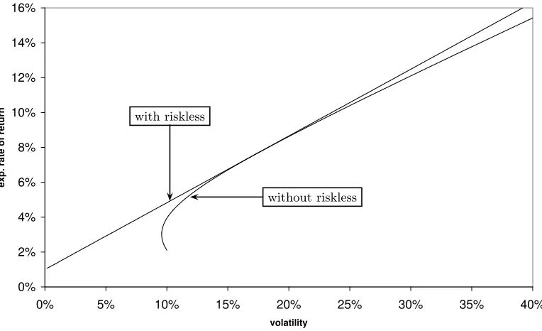
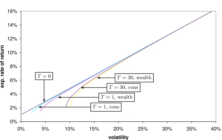
A riskless asset corresponds to a point (0, r) in the (standard deviation, mean)-diagram. The investors can combine any portfolio of risky assets with an investment in the riskless asset. The (standard deviation, mean)-pairs that can be obtained by such a combination forms a straight line between the point (0, r) and the point corresponding to the portfolio of risky asset. Other things equal, greedy and risk-averse investors want high expected return and low standard deviation so they will move as far to the “north-east” as possible in the diagram. Consequently they will pick a point somewhere on the upward-sloping line that is tangent to the mean-variance frontier of risky assets and goes through the point (0, r). The point where this line is tangent to the frontier of risky assets corresponds to a portfolio which we refer to as the tangency portfolio. This is a portfolio of risky assets only. It is the portfolio that maximizes the Sharpe ratio over all risky portfolios. The Sharpe ratio of a portfolio is the ratio (µ(π)−r)/σ(π) between the excess expected return of a portfolio and the standard deviation of the return. The tangency portfolio is given by the portfolio weights
πtan= 1
1>Σ−1(µ−r1)Σ−
1(µ
−r1). (3.10)
This upward-sloping straight line constitutes the mean-variance frontier of all assets. Again it is quite cumbersome to compute exactly which of these mean-variance efficient portfolios that a given investor prefers, except for the case of negative exponential utility. Again we have two-fund separation since all investors will combine just two funds, where one fund is simply the riskless asset and the other is the tangency portfolio.
3.3 Critique of the one-period framework 20
3.3
Critique of the one-period framework
• Investors typically get utility from consumption at different points in time and not simply the wealth level at one particular date.
• Even in the case where the investor only obtains utility from wealth at one date, she has the opportunity to change her portfolio over time, which she would normally do as new information arises (e.g. when stock prices and interest rates change) or simply because time passes. Investors live in a dynamic model and will take decisions dynamically. Of course, the existence of transaction costs is a reason for not changing the portfolio too frequently, but if we are really worried about transaction costs we should explicitly model that imperfection – the analysis of such models is quite difficult, however.
• Consumption and investment decisions are generally not to be separated from each other. Investments are meant to generate future consumption!
Chapter 4
Introduction to multi-period models
To study dynamic consumption and investment decisions, several papers have looked at multi-period, discrete-time models where the investor has the opportunity to consume and rebalance her portfolio at a number of fixed dates. Certainly this is a valuable extension of the single-period setting, but it is still a limitation that the investor can only change her decisions at pre-specified points in time and not react to new information arriving between these points in time. A continuous-time model seems more reasonable. Furthermore, the results on optimal consumption and investment strategies are typically clearer in continuous-time models than in discrete-time models, and the necessary mathematical computations are much more elegant in a continuous-time framework. Therefore, we will not give much attention to multi-period, discrete-continuous-time models. However, some aspects of the set-up of continuous-time models may be easier to understand if we start by looking at a discrete-time model and then take the limit as the period length goes to zero. The basic references for the discrete-time models are Samuelson (1969), Hakansson (1970), Fama (1970, 1976), and Ingersoll (1987, Ch. 11).
4.1
A multi-period, discrete-time framework
Consider the time line below:
t0≡0
∆t t1
∆t
t2 tN−1
∆t
tN ≡T
At time tn = n∆t for n = 0,1, . . . , N −1 the investor chooses a portfolio θtn which is held unchanged until time tn+1 and a consumption rate ctn such that the total consumption in the interval [tn, tn+1) is ctn·∆t. (We assume that there is a single consumption good so that ctn is one-dimensional.) This is subtracted from her wealth at time tn. Of course, θtn and ctn can only be based on the information known at time tn, i.e. in mathematical terms they must be
Ftn-measurable. We assume that there is no consumption or investment beyond time T, which we can think of as the time of death (assumed to be known in advance!). At time 0 the investor must choose the entire consumption rate processc0, ct1, . . . , ctN−1 and the entire portfolio process θ0, θt1, . . . , θtN−1. In other words, she must choose the current valuesc0 andθ0and for each future
4.2 Wealth dynamics 22
date tn (with n= 1, . . . , N −1) she must choose a consumption rate ctn(ω) andθtn(ω) for each possible state of the worldωat day tn.
We assume that the life-time utility of consumption and terminal wealth is given by
U(c0, c1, . . . , cT, WT) = T
X
t=0
e−δtu(ct) +e−δTu¯(W T)
as discussed in Section 2.4. The maximal obtainable expected life-time utility seen from time 0 is therefore
J0= sup (ctn,θtn)Nn=0−1
E
"N−1 X
n=0
e−δtnu(c
tn)∆t+e
−δTu¯(W T)
#
,
where the supremum is taken over all budget-feasible consumption and investment strategies. Similarly, we define
Jti = sup
(ctn,θtn)N
−1
n=i Eti
"N−1 X
n=i
e−δ(tn−ti)u(c
tn)∆t+e
−δ(T−ti)u¯(W T)
#
, i= 0, . . . , N−1, (4.1)
where the subscript on the expectations operator denotes that the expectation is taken conditional on the information known to the agent at timeti. J is often called the indirect or derived utility of wealth process or function, since it measures the highest attainable expected life-time utility the investor can derive from her current wealth in the current state of the world.
4.2
Wealth dynamics
Denote by Ptn = (P
1
tn, . . . , P d tn)
> the vector of prices of the d risky assets at time tn. The
nominal riskfree rate of return per year in the period [tn, tn+1) is denoted byrtn. This means that the riskfree rate of return over the period is rtn∆t. The value at timetn of a dollar invested at time 0 and subsequently rolled over at the riskfree rate is denoted byP0
tn. We will refer to such a unit bank account as asset 0. For the purposes of deriving the budget constraint we will represent the portfolio by the number of units of each asset held. We letNi
tn denote the number of units of asseti= 0,1, . . . , dheld in the period [tn, tn+1). We will allow for the case where the agent earns
income from other sources than his financial investments. We letytnbe the rate of income earned in the period [tn, tn+1) such that the entire income in this period is ytn ·∆t. We assume that the agent receives this amount at timetn. Note that we do not model the labor supply decision resulting in this income, but takeytn as exogenously given.
The agent enters datetn with a wealth of
Wtn= d
X
i=0
Ntin−1P
i tn.
This is the value of her portfolio chosen in the previous period. She then receives incomeytn·∆tand simultaneously has to choose the consumption ratectn and the new portfolio (N
0
tn, N
1
tn, . . . , N d tn). The budget restriction on these choices is that
(ytn−ctn) ∆t= d
X
i=0
h
Ntin−N i tn−1
4.3 Dynamic programming in discrete-time models 23
i.e. that income net of consumption equals the extra amount invested in the financial market. We then get that
Wtn+1−Wtn= d
X
i=0
NtinP i tn+1−
d
X
i=0
Ntin−1P
i tn = d X i=0
Ntin
Ptin+1−P
i tn + d X i=0 h
Ntin−N i tn−1
i Ptin
= d X i=0 Ni tn Pi
tn+1−P
i tn
+ (ytn−ctn) ∆t.
Letθi tn =N
i tnP
i
tn denote the amount invested in asset iand letR i tn=
Pi
tn+1−P
i tn
/Pi
tn denote the rate of return on asseti. Then the change in wealth can be rewritten as
Wtn+1−Wtn = d
X
i=0
θitnR i
tn+ (ytn−ctn) ∆t.
With the vector notationθtn= (θ
1
tn, . . . , θ d tn)
>andR
tn= (R
1
tn, . . . , R d tn)
>, we get
Wtn+1−Wtn=θ
0
tnrtn∆t+θ >
tnRtn+ (ytn−ctn) ∆t.
Note that the only stochastic variable (seen from time tn) on the right-hand side is the return vectorRtn. Let us decompose the return into an expected and an unexpected part,
Rtn =µtn∆t+σtnεtn
√
∆t. (4.2)
Hereµtnis the vector of expected rates of return per year,εtn is a vector of independent stochastic shocks all with mean zero and variance one, and σtn is a matrix determining how the returns are affected by these shocks. The values of µtn and σtn are known at time tn. The realization of the shock vectorεtn will be known at time (n+ 1)∆t, just before the consumption and portfolio decisions at that date are taken. It follows that, seen at timetn, the variance-covariance matrix of
Rtn is given byσtnσ >
tn∆t. The elements in Σtn ≡σtnσ >
tn are hence variances and covariances per year. The change in wealth can now be rewritten (yet another time) as
Wtn+1−Wtn=
θt0nrtn+θ >
tnµtn+ytn−ctn
∆t+θ>
tnσtnεtn
√
∆t. (4.3)
4.3
Dynamic programming in discrete-time models
4.3 Dynamic programming in discrete-time models 24
This result is based on the following manipulations:
Jti= sup
(ctn,θtn)Nn=−i1 Eti
"N−1 X
n=i
e−δ(tn−ti)u(c
tn)∆t+e
−δ(T−ti)u¯(W T)
#
= sup
(ctn,θtn)N
−1
n=i Eti
"
u(cti)∆t+ N−1
X
n=i+1
e−δ(tn−ti)u(c
tn)∆t+e
−δ(T−ti)u¯(W T)
#
= sup
(ctn,θtn)N
−1
n=i Eti
"
u(cti)∆t+ Eti+1 "N−1
X
n=i+1
e−δ(tn−ti)u(c
tn)∆t+e−
δ(T−ti)u¯(W T)
##
= sup
(ctn,θtn)Nn=−i1 Eti
"
u(cti)∆t+e
−δ∆tEt i+1
"N−1 X
n=i+1
e−δ(tn−ti+1)u(c
tn)∆t+e
−δ(T−ti+1)u¯(W
T)
##
= sup cti,θti
Eti
"
u(cti)∆t+e
−δ∆t sup
(ctn,θtn)N
−1
n=i Eti+1
"N−1 X
n=i+1
e−δ(tn−ti+1)u(c
tn)∆t+e
−δ(T−ti+1)u¯(W
T)
##
Here, the first equality is simply due to the definition of indirect utility, the second equality comes from separating out the first term of the sum, the third equality is valid according to the law of iterated expectations, the fourth equality comes from separating out the discount term
e−δ∆t, and the final equality is due to the fact the only the inner expectation depends on future consumption rates and portfolios. Noting that the inner supremum is by definition the indirect utility at timeti+1, we arrive at
Jti = sup cti,θti
Eti
u(cti)∆t+e− δ∆tJ
ti+1
. (4.4)
This equation is called the Bellman equation, and the property is called the dynamic
pro-gramming property. The decision to be taken at timetnis split up in two: (1) the consumption
and portfolio decision for the current period and (2) the consumption and portfolio decisions for all future periods. We take the decision for the current period assuming that we will make optimal decisions in all future periods. Note that this does not imply that the decision for the current pe-riod is taken independently from future decisions. We take into account the effect that our current decision has on the maximum expected utility we can get from all future periods. The expectation Eti
Jti+1
will depend on our choice ofcti andθti.
The dynamic programming property is the basis for a backward iterative solution procedure. First, we choosectN−1 and θtN−1 to maximize
u(ctN−1)∆t+e −δ∆tEt
N−1[¯u(WT)],
where
WT =WtN−1+ h
θ0tN−1rtN−1+θ >
tN−1µtN−1+ytN−1−ctN−1 i
∆t+θ>
tN−1σtN−1εtN−1
√ ∆t.
This is done for each possible state at time tN−1 and gives usJtN−1. Then we choose ctN−2 and θtN−2 to maximize
u(ctN−2)∆t+e −δ∆tEt
N−2
JtN−1
,
4.4 The basic continuous-time setting 25
are expected to depend on the wealth level of the agent at that date, but also on the value of other time-varying state variables that affect future returns on investment (e.g. the interest rate level) and future income levels. To be practically implementable only a few state variables can be incorporated. Also, these state variables must follow Markov processes so only the current values of the variables are relevant for the maximization at a given point in time. Note the similarity to the problem of determining the optimal exercise strategy of a Bermudan/American option. However, for that problem the decision to be taken is much simpler (exercise or not) than for the consumption/portfolio problem.
Under some simplifying assumptions on the precise form of the utility functionsuand ¯uand on the dynamics of asset returns and income, the backward iterative procedure yields an explicit solu-tion to the maximizasolu-tion problem in the form of the optimal (possibly state- and time-dependent) consumption rate and portfolio process (and also the indirect utility of wealthJt). Since we can ob-tain similar (and often clearer) results under similar assumptions in the more elegant and realistic continuous-time setting, we will not go into these discrete-time examples.
4.4
The basic continuous-time setting
The basic elements of mainstream continuous-time models can be seen as the limit of the multi-period discrete-time model elements. The basis is a probability space (Ω,F,P) with an associated filtrationF= (Ft)t∈[0,T] which is the formal model of the evolution of the relevant uncertainty for
the investor.
The agent now has to choose a continuous-time process of consumption rates c = (ct)t∈[0,T]
and a continuous-time portfolio processθ= (θt)t∈[0,T]. As before,θtis thed-dimensional vector of amounts invested at timetin thedrisky assets. The remaining financial wealthθ0t =Wt−θt>1=
Wt−Pdi=1θit is invested in the locally riskfree asset. A single consumption good is assumed and this good is used as a numeraire so that all prices are measured in units of this consumption good, i.e. in real terms. We will always require that ct ≥ 0 with probability one. We focus on unconstrained investors so that there are no constraints on the valuesθtmay have, i.e.θtcan have any value inRd; see references in Section 10.2 to problems with constraints on the portfolios, e.g. short-selling constraints or portfolio mix constraints. The stochastic variablesct and θt must be
Ft-measurable, i.e. they can only depend on information available at time t. In other words, the processesc andθ are adapted. Other technical requirements should be added.1 A consumption
and investment strategy must also satisfy that the wealth process induced by the strategy always stays above a lower bound, say −K, where K > 0. This rules out doubling strategies, cf. the discussion in Duffie (2001, Ch. 6). In fact, we will typically require that wealth stays non-negative at all times. This is a natural requirement, at least for the case where the investor does not receive a minimum income from non-financial sources (labor). The set of all consumption and investment strategies that satisfy all these requirements on the interval [t, T] is denoted byAt.
1 The consumption processc must be anL1-process, i.e. RT
0 kctkdt <∞with probability one. The portfolio
strategyθmust satisfy thatθ>µis anL1-process and thatθ>σis anL2-process, i.e. thatRT
4.4 The basic continuous-time setting 26
Preferences: The objective is to maximize the expected life-time utility which is assumed to be
on the additively time-separable form
E
"Z T
0
e−δtu(ct)dt+e−δTu¯(W T)
#
, (4.5)
where uand ¯u are increasing and concave von Neumann-Morgenstern utility functions. We will assume that u and ¯u are twice continuously differentiable on their domain. We will define the indirect utility processJ= (Jt) as
Jt= sup
(c,θ)∈At Et
"Z T t
e−δ(s−t)u(cs)ds+e−δ(T−t)u¯(W
T)
#
. (4.6)
An optimal consumption and investment strategy (c∗, θ∗) has the property that it provides at least
as high an expected life-time utility as any other feasible strategy. In particular,
J0= E
"Z T
0
e−δtu(c∗t)dt+e−δTu¯(WT∗)
#
,
where W∗
T is the terminal wealth level that follows from the strategy (c∗, θ∗). In other words, when an optimal strategy exists the supremum in the definition ofJ is attained. Of course,J0 will
depend on the initial wealthW0 of the investor. We shall assume thatJ0<∞for allW0<∞. It
can be shown thatJ0is an increasing and concave function of initial wealthW0. See Exercise 4.1
at the end of the chapter.
Dynamics of prices and wealth: When the investor is about to choose consumption and
investment strategies she has to deal with a number of variables that can evolve stochastically over time such as:
• the (locally) riskfree ratert(i.e. the short-term interest rate),
• the prices, the expected rates of returns, the variance-covariance matrix of rates of return on the risky assets,
• the expected rate of change and variation in her income rate, • covariances or correlations between all these variables.
Of course, in a fuller model we should also include uncertainty e.g. about the time of death of the investor, relative prices of different consumption goods, etc., but we ignore these issues at this point.
We shall assume that all exogenous shocks to these variables can be represented by standard Brownian motions. A direct consequence is that we do not allow for any jumps in prices, except for points in time where the asset provides its owner with a lump-sum payment, e.g. a dividend payment of a stock or a coupon payment of a bond.2 For simplicity, we assume that the assets
provide no payments in the life of the investor and that the vector of risky asset pricesPt follows a stochastic process of the form
dPt= diag(Pt) [µtdt+σtdzt], (4.7)
2See, e.g., Bardhan and Chao (1995), Wu (2000), and Jeanblanc-Picqu´e and Pontier (1990) for utility