Time derivative of the horizontal geomagnetic field as an activity indicator

Annales

Geophysicae

Time derivative of the horizontal geomagnetic field as an activity

indicator

A. Viljanen1, H. Nevanlinna1, K. Pajunp¨a¨a1, and A. Pulkkinen1

1_{Finnish Meteorological Institute, Geophysical Research Division, P.O. Box 503, FIN-00101 Helsinki, Finland} Received: 20 February 2001 – Revised: 12 June 2001 – Accepted: 10 June 2001

Abstract. Geomagnetically induced currents (GICs) in technological conductor systems are a manifestation of the ground effects of space weather. Large GICs are always as-sociated with large values of the time derivative of the ge-omagnetic field, and especially with its horizontal compo-nent (dH/dt). By using the IMAGE magnetometer data from northern Europe from 1982 to 2001, we show that large

dH/dt’s (exceeding 1 nT/s) primarily occur during events governed by westward ionospheric currents. However, the directional distributions ofdH/dtare much more scattered than those of the simultaneous baseline subtracted horizontal variation field vector∆H. A pronounced difference between

∆HanddH/dttakes place at about 02–06 MLT in the au-roral region whendH/dtprefers an east–west orientation, whereas∆Hpoints to the south.

The occurrence of largedH/dthas two daily maxima, one around the local magnetic midnight, and another in the morn-ing. There is a single maximum around the midnight only at the southernmost IMAGE stations. An identical feature is observed when large GICs are considered. The yearly num-ber of largedH/dtvalues in the auroral region follows quite closely theaaindex, but a clear variation from year-to-year is observed in the directional distributions. The scattering of

dH/dtdistributions is smaller during descending phases of the sunspot cycle. Seasonal variations are also seen, espe-cially in winterdH/dtis more concentrated to the north– south direction than at other times.

The results manifest the importance of small-scale struc-tures of ionospheric currents when GICs are considered. The distribution patterns ofdH/dtcannot be explained by any simple sheet-type model of (westward) ionospheric currents, but rapidly changing north-south currents and field-aligned currents must play an important role.

Key words. Geomagnetism and paleomagnetism (geomag-netic induction; rapid time variations) - Ionosphere (iono-spheric disturbances)

Correspondence to: A. Viljanen ([email protected])

1 Introduction

Geomagnetically induced currents (GIC) in power systems, pipelines and other technological conductor systems on the ground occur during rapid changes in the Earth’s magnetic field (e.g. Boteler et al., 1998; Viljanen and Pirjola, 1994). However, little attention has been paid to the ionospheric current systems, which primarily produce GIC. Somewhat inexact terminology appears in literature linking GIC to elec-trojets, which flow approximately parallel to the (magnetic) east–west direction. In particular, this has often led to a con-sideration of oversimplified electrojets models, which im-plicitly or exim-plicitly imply that the electric field driving GIC is primarily east–west oriented (e.g. Albertson et al., 1981; Boteler et al., 1997; Towle et al., 1992; Viljanen and Pir-jola, 1994). A further inference has been that, for example, power lines parallel to geomagnetic latitudes are most prone to induction effects. A more general problem is to character-ize the ionospheric current systems which can produce large GIC.

When the GIC problem is considered from the modelling viewpoint, the key quantity is the horizontal geoelectric field associated with geomagnetic variations. However, the elec-tric field is seldom directly measured. On the other hand, GIC is closely related to the time derivative of the magnetic field (dB/dt), or more exactly, to its horizontal part (Coles et al., 1992; M¨akinen , 1993; Viljanen, 1998). Further evidence about this is given by Bolduc et al. (1998) who related the measured electric field to the time derivative of the orthog-onal horizontal magnetic field. Therefore, we can base our investigation on the ground magnetic field which is available from several sites during long periods.

larger data set and a more illustrative new way by studying directional distributions of the horizontal variation field vec-tor and its time derivative. The temporal occurrence of large time derivatives will be considered from hourly to solar cycle scales.

There are several previous statistical investigations on ge-omagnetic variations at high latitudes based on the AU, AL and AE indices, with the most recent papers by Hajkowicz (1998) and Ahn et al. (2000). Our study is significantly dif-ferent from theirs, because our data selection is based on the time derivative of the magnetic field, and not on the ampli-tude of variations. Furthermore, we concentrate on a local scale.

Among others, Olson (1986), Vennerstrøm (1999), and Ziesolleck and McDiarmid (1995) have studied ULF tions at high latitudes. Due to the equivalence of field varia-tions and their time derivatives in the frequency domain, their results can also be interpreted in terms ofdB/dt. Although these authors have not based their event selections on the am-plitude, there are some similarities to our results which will be discussed in this paper.

The structure of this paper is as follows: after briefly de-scribing the data selection (Sect. 2.1), we present results from five stations in the average auroral region using a long-term data series (Sect. 2.2). A comparison between the horizontal field and its time derivative during a shorter period, but in a larger region is given in Sect. 2.3 with some remarks about seasonal variations (Sect. 2.4). The effect of the Earth’s con-ductivity anomalies is discussed in Sect. 2.5. Finally, results based on GIC recordings are shown in Sect. 2.6.

2 Directional distributions of the horizontal magnetic field and its time derivative

2.1 Selection of data

We use data from the IMAGE magnetometer network (Fig. 1) in Fennoscandia and Svalbard (Syrj¨asuo et al., 1998), and also from the preceding EISCAT magnetometer cross (L¨uhr et al., 1984). A reference to measured GICs will be made as well.

When studying the baseline subtracted horizontal varia-tion field vector (∆H = ∆Xex+ ∆Yey), we select such timesteps that|dH/dt|>1 nT/s, where the time derivative is calculated by subtracting successive values and dividing by the sampling interval (we use the simple notationdH/dt, because the time derivative does not depend on baselines). In terms of GIC, 1 nT/s typically causes a current of a few am-peres in the Finnish high-voltage power system or the natural gas pipeline.

An approximate rule for interpreting vector distributions is that∆Hcan be converted to an overhead equivalent iono-spheric current by a 90◦ clockwise rotation. WhendH/dt

is rotated 90◦ anticlockwise, it is parallel to the horizontal electric field at the Earth’s surface (strictly true in the

fre-0° 20° 40°

75°

70°

65°

60°

BJN NAL

HOP HOR

NUR NO

RW AY

SW ED

EN

FINLAND RUSSIA

LOZ SOD

TRO

PEL

OUJ

HAN MUO SOR

KEV MAS KIL

UPS LYC RVK

DOB

LYR

KIR ABK AND

LEK

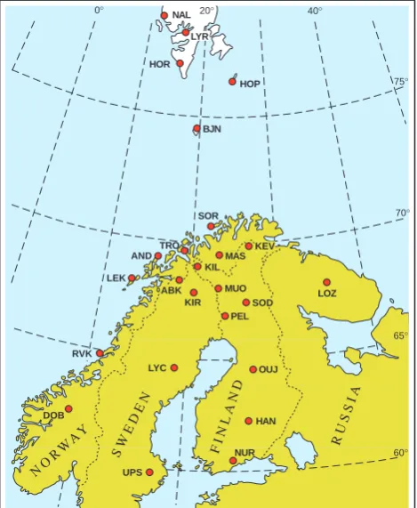
Fig. 1. IMAGE magnetometer stations in 2000. Geographic lati-tudes and longilati-tudes are shown in the figure. Geomagnetic latilati-tudes are approximately obtained by subtracting 3◦from the geographic ones.

quency domain if the disturbance field is a plane wave and the Earth’s conductivity depends only on depth).

In the following, we primarily ignore stations in Sval-bard, because they are located at latitudes farther north of all ground technological systems which presently can expe-rience GIC.

2.2 Distributions ofdH/dtin the auroral region

SOR 6544 1982 19223 1983 24592 1984 18367 1985 20091 1986 13810 1987 14500 1988 28875 1989 15256 1990 28606 1991 20956 1992 25369 1993 47364 1994 17881 1995 13067 1996 8525 1997 14711 1998 19290 1999 13330 2000 KEV 10487 1983 18034 1984 15961 1985 14691 1986 10554 1987 11508 1988 24070 1989 16568 1990 27323 1991 17016 1992 23217 1993 28690 1994 16911 1995 9557 1996 8562 1997 13799 1998 15565 1999 17187 2000 KIL 11581 1983 34041 1984 10303 1985 11621 1986 6370 1987 14095 1988 31469 1989 21577 1990 36307 1991 21781 1992 27276 1993 46208 1994 19981 1995 11062 1996 8475 1997 15677 1998 19180 1999 21154 2000 MUO 6542 1982 23839 1983 21887 1984 10912 1985 12905 1986 8319 1987 10548 1988 26961 1989 16587 1990 29823 1991 17622 1992 20730 1993 35446 1994 13247 1995 6367 1996 7259 1997 13944 1998 14961 1999 13991 2000 PEL 16217 1983 16355 1984 6972 1985 10178 1986 5582 1987 8578 1988 23419 1989 15292 1990 29519 1991 16342 1992 15712 1993 25689 1994 10059 1995 4635 1996 6072 1997 11134 1998 11179 1999 15804 2000

Fig. 2. Directional distributions ofdH/dtat Sørøya (SOR), Kevo (KEV), Kilpisj¨arvi (KIL), Muonio (MUO) and Pello (PEL) from 1982 to 2000. Only timesteps fulfilling the condition|dH/dt|>

1 nT/s are included. The sampling interval was 20 s until November 1992, and after that 10 s. For consistency, 10 s values were averaged to 20 s. The eleven years of the sunspot cycle 22 are in the middle row. The geographic north direction is upwards. The distribution patterns are normalized separately for each year for better readabil-ity. The number of timesteps is given under each subplot. Data from 1982 to 1983 were available only of short periods, and only about half of 1985 to 1987 was covered at KIL. The geomagnetic latitudes of the stations are between 63◦and 67◦.

1982 1984 1986 1988 1990 1992 1994 1996 1998 2000

0 1 2 3 year datapoints [%]

PEL, MUO, KIL, KEV, SOR

10 20 30 40

aa

PEL MUO KIL KEV SOR

0 0.5 1 1.5 2 datapoints [%] 1982-2000

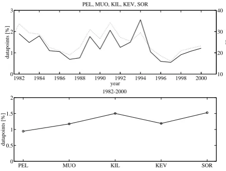
Fig. 3. Relative number of datapoints used in Fig. 2. Upper panel: yearly average of all five stations; the dotted line is the yearly aver-age of the aa index (obtained from the National Geophysical Data Center). Lower panel: average value at stations from 1982 to 2000. The sampling interval used here is 20 s, which was the original one for data from 1982 to 1992. The newer 10 s data were averaged to 20 s values too.

transient. Transient storms are usually more intense, but how this affectsdH/dtdistributions is unclear.

The relative number of datapoints with|dH/dt|>1nT/s compared to theaaindex is shown in Fig. 3. The relative number of points at each station (lower panel) is larger at KIL than at KEV, although they are approximately at the same magnetic latitude. The possibility that this is caused by the Earth’s conductivity will be discussed in Sect. 2.5. The yearly occurrence correlates well with the aa index. Some periodicity is seen, with the smallest number (1987, 1997) occurring a little after the minimum of the sunspot cy-cle (1986, 1996). However, it is peculiar that in both 1987 and 1994 one can see narrow distributions in Fig. 2, although theirdH/dtactivity levels are the smallest and highest ones in Fig. 3. The least and most scattered years (1987, 1998) are separated by 11 years, i.e. one solar cycle.

Vennerstrøm (1999) considered the power spectral density of 2–4 min, and the 5–10 min frequency bands of the Green-land magnetometer chain during the morning hours (06– 10 MLT). She found a good correlation between the power spectral density andaaat the southern stations of the chain, located at about the same magnetic latitudes as the five sta-tions in Fig. 2. This result is clearly equivalent to that shown in the upper panel of Fig. 3 since large dH/dtvalues are associated with short-period variations. The similarity is in-teresting since we have considered all local times, and Ven-nerstrøm (1999) considered only the local morning, which primarily lacks, for example, substorm activity. However, as will be seen in Sect. 2.3, the local morning hours have a sig-nificant contribution to the total number of largedH/dtat auroral latitudes.

indices are presented by Hajkowicz (1998) and Ahn et al. (2000). However, any evident correlation to the variability of

dH/dtis hard to find due to the very different data selection criteria compared to our study.

According to these results, a considerable variation of the

dH/dtdistributions from year-to-year, and from site-to-site, is a clear fact. Next, it is interesting to study the simultaneous distributions of the horizontal variation field∆H.

2.3 Distribution of∆HanddH/dtat all IMAGE stations Our basic dataset for the∆H investigation consists of all available values from 1994 to 2000 at the IMAGE mag-netometer stations (with the condition|dH/dt| > 1nT/s). Since we currently study field variations, quiet time baselines are needed. They have been selected visually and separately for each day. Although this is somewhat subjective, for the present purpose, small uncertainties are unimportant (time derivatives do not depend on baselines). For computational convenience, we now consider one minute values.

An example of distributions at Kilpisj¨arvi (KIL) located in the average auroral zone, and Ouluj¨arvi (OUJ) in the subau-roral region is shown in Fig. 4, where the distribution patterns are normalized separately for each subplot. The main direc-tion of∆H is to SSE, which is equivalent to an overhead WSW directed ionospheric current parallel to the local ge-omagnetic latitude. The eastward electrojet has a relatively significant contribution only during some years and only at the southernmost sites. The directional distribution of∆H is nearly identical from year-to-year, whereas the distribution ofdH/dtclearly varies.

The number of included timesteps with 20 s values is 5 to 6 times that of one minute values (Figs. 2 and 4). In addition to the larger number of 20 s datapoints, one-minute averaging smooths out many spikes. However, yearly distributions of

dH/dtdo not change much. Concerning∆Hdistributions, it does not matter whether 10 s or 20 s or one minute data are used.

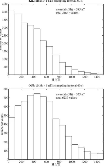
Most timesteps of large|dH/dt| are associated with ac-tive periods, as shown by the distributions of|∆H|depicted in Fig. 5. When all available one-minute values from 1994 to 2000 are used, the average|∆H|is 33 nT at OUJ, and 60 nT at KIL, which are much smaller than the ones in Fig. 5. The difference in the shape of the distributions between KIL and OUJ indicates that large|dH/dt|values at subauroral lati-tudes are more regularly associated with exceptionally large geomagnetic variations. This is the case at all subauroral IM-AGE stations.

Directional distributions of∆HanddH/dtat the conti-nental IMAGE stations are presented in Fig. 6. This example concerns the year 2000 when there were 25 stations operat-ing, and the solar cycle maximum was reached. The com-mon feature of∆Hat all sites is its narrow orientation along the local magnetic meridian to SSE. The time derivative is more varying, although there is a clear concentration along the NNW-SSE line at subauroral sites. The tilted dH/dt

pattern due to a conductivity anomaly at LYC will be

dis-1994

7737 1995

3300 1996

1711 1997

1573 1998

2751 1999

3555 2000

4040 KIL: directional distribution of H (dH/dt > 1.0 nT/s)

sampling interval 60 s

directional distribution of dH/dt

1994

1463 1995

519 1996

77 1997

506 1998

1368 1999

685 2000

1619 OUJ: directional distribution of H (dH/dt > 1.0 nT/s)

sampling interval 60 s

directional distribution of dH/dt

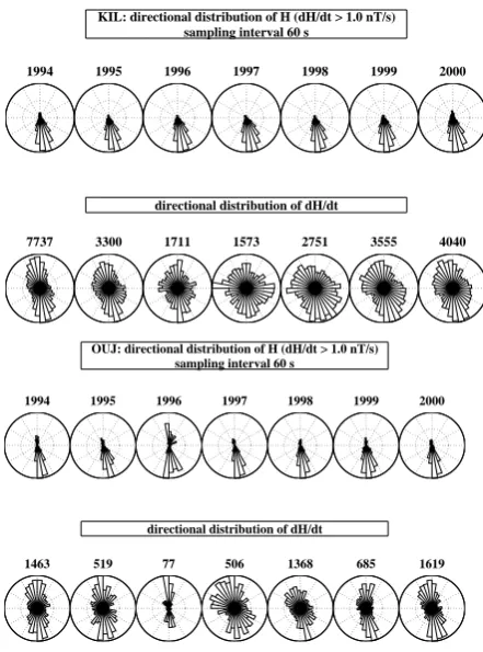
Fig. 4. Directional distribution of∆H (upper row) anddH/dt

(lower row) at Kilpisj¨arvi (KIL) and Ouluj¨arvi (OUJ) from 1994 to 2000, as calculated from one minute values. Only timesteps fulfill-ing the condition|dH/dt|>1nT/s are included. The distribution patterns are normalized separately for each subplot. The total num-ber of timesteps are given as title texts in the lower row.

cussed in Sect. 2.5. Data from LOZ in 2000 is not shown due to an instrumental problem which biased the statistical results. Inspection of earlier years showed that LOZ resem-bles SOD and PEL, which are approximately located at the same geomagnetic latitude.

For clarity, the vector distributions are scaled separately for each site in Fig. 6. The relative number of large values is illustrated in Fig. 7. It is smallest at southern sites and then increases northward. The relative numbers at the Svalbard stations (not shown in the figure) are 0.75% (BJN), 0.80% (HOP), 0.66% (HOR), 0.39% (LYR), and 0.22% (NAL), so thedH/dtactivity decreases northward of the average au-roral region. This behaviour is typical for all local times, as also shown by Boteler et al. (1997) when considering the oc-currence of hourly maxima ofdX/dtover 1 nT/s in Canada. We also calculated the daily sum of large|dH/dt|values at all IMAGE stations and compared it to the Ak index of Nurmij¨arvi. The correlation coefficient between these two activity indicators varies between 0.71–0.87 from 1994 to 2000. Consequently, the daily activity can be described in terms of|dH/dt|as well.

0 200 400 600 800 1000 1200 1400 0

500 1000 1500 2000 2500 3000 3500 4000 4500

H [nT]

number of values

KIL: dH/dt > 1 nT/s (sampling interval 60 s)

mean(abs(H)) = 385 nT total 24667 values

0 200 400 600 800 1000 1200 1400

0 100 200 300 400 500 600 700 800

H [nT]

number of values

OUJ: dH/dt > 1 nT/s (sampling interval 60 s)

mean(abs(H)) = 523 nT total 6237 values

Fig. 5. Distribution of the amplitudes of the∆Hvectors used in Fig. 4. When all available values from 1994 to 2000 are used, the averages are 33 nT at OUJ and 60 nT at KIL.

in 2000 is presented in Fig. 8. The magnetic local time (MLT) used here is the one associated with the solar mag-netic coordinate system. It is obtained from the GSM system by a rotation around the y axis so that z is parallel to the dipole axis. The difference between UT and MLT was sim-ply taken as an average of the whole year for each station separately. For statistical purposes this is sufficiently accu-rate (the solar MLT is 10–20 minutes ahead of the CGM MLT in the mainland stations). Only the year 2000 is shown here, but we also calculated the corresponding results from 1994 to 1999, which basically have a similar behaviour.

The diurnal behaviour at the auroral region (KIL) is con-sistent with the directional distribution of ∆H, in which the nighttime westward electrojet dominates. The midnight maximum can be related to the substorm activity, and the morning peak can be related at least partly to pulsations and omega bands. Typical pulsations such as Pc5’s with periods of 150–600 s and amplitudes of 100 nT, can produce|dH/dt| up to2π100/150nT/s≈4nT/s.

The double peak in Fig. 8 is most pronounced at stations in the average auroral region, which is in accordance with the

directional distribution

H (dH/dt > 1.0 nT/s) 366 events (2000) sampling interval 60 s

UPS

NUR HAN DOB

OUJ LYC

RVK

PEL SOD

KIR MUO

ABK LEK

KIL

AND MAS

TRO KEV

SOR

directional distribution

dH/dt (dH/dt > 1.0 nT/s) 366 events (2000) sampling interval 60 s

-800 -600 -400 -200 0 200 -600

-400 -200 0 200 400

0.06 %

0.10 % 0.13 % 0.14 %

0.31 % 0.55 %

0.46 %

0.59 % 0.56 % 0.62 % 0.57 % 0.84 %

0.52 %

0.79 % 0.72 % 0.91 % 0.86 %

0.75 % 0.75 %

y [km]

x [km]

relative number of values

dH/dt > 1.0 nT/s 366 events (2000) sampling interval 60 s

Fig. 7. Relative number of data points fulfilling the condition |dH/dt| > 1nT/s at each station in Fig. 6. The radius of each circle is proportional to the percentage.

results of Coles and Boteler (1993), Boteler et al. (1997) (re-plotted in Boteler et al., 1998). ULF studies also reveal the same feature (e.g. Vennerstrøm, 1999; Ziesolleck and McDi-armid, 1995); the years 1996 and 1997 even have a slight triple structure. At the southernmost sites (UPS, NUR), the early morning minimum is sometimes missing (e.g. 2000), but at times, it is observable (e.g. 1998). The double peak was also found by Viljanen (1997) in terms of the average value ofdB/dt, but he did not discuss the subject further.

At the Svalbard stations the morning maximum typically occurs around 10 MLT (latest in the north, as found by Boteler et al., 1997, as well) and the evening maximum just before the local midnight, as at more southern latitudes, but the variability from year-to-year is large. Furthermore, there are often three clearly distinct maxima, as at LYR in 2000. Olson (1986) studied Pc3-5 pulsations at Cape Perry (mag-netic latitude about 74◦) and found the occurrence maxima at about 9 MLT and 19 MLT, i.e. somewhat earlier than at LYR (magnetic latitude 75).

Although ULF studies show that variations in certain fre-quency bands have the same daily occurrence probability, some care will be needed in the interpretation. As mentioned by Vennerstrøm (1999), it is not possible to distinguish the ULF band power due to different physical phenomena, such as broadband noise, Pi and Pc pulsations, impulse events and substorm expansions. Therefore, in future studies, quantita-tive models of ionospheric currents during large GIC events are needed.

Nevanlinna and Pulkkinen (2001) have studied the

diur-0 5 10 15 20

0 50 100 150

MLT [h]

#

timesteps with dH/dt > 1.0 nT/s at LYR (year 2000)

0 5 10 15 20

0 50 100 150 200 250 300 350 400 450

MLT [h]

#

timesteps with dH/dt > 1.0 nT/s at KIL (year 2000)

0 5 10 15 20

0 10 20 30 40 50 60 70

MLT [h]

#

timesteps with dH/dt > 1.0 nT/s at NUR (year 2000)

nal occurrence of auroras in north Finland using all-sky cam-era data from 1973 to 1997. The mean hourly occurrence of auroras has nearly a Gaussian distribution centered at the local magnetic midnight. The probability of seeing auroras is slightly higher in the morning hours, but a double peak, such as the one at the auroral region station KIL in Fig. 8, does not exist. There is a double peak, although it is not very pronounced, only when the auroral occurrence is considered during rare severe storms. In addition, these maxima are at about 16 and 04 MLT, which differ from those of|dH/dt|.

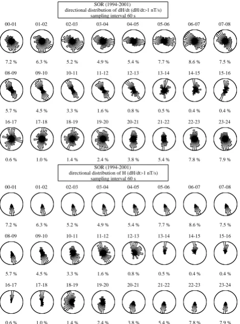
We also calculated the hourly distribution for a few sta-tions, of which SOR is shown as an example in Fig. 9. Each hourly pattern is again normalized separately, and the relative number of datapoints is given under each subplot. A very similar behaviour was found at MUO as well. Although the selection of data is based on the large|dH/dt|condition, the H distribution reflects the familiar diurnal pattern of iono-spheric currents. The daytime convection (8–16 MLT) with the turning of the electrojet from the westward to the east-ward direction is clear (11–13 MLT). The Harang disconti-nuity at 18–20 MLT is also distinctly manifested with the ro-tation of the∆Hpattern from the north to the south through the west. The rest of the time is governed by westward cur-rents.

The dH/dt vector follows in many respects what one could expect: in the daytime and in the evening, before mid-night, it is primarily parallel (or antiparallel) to∆H. How-ever, after midnight, until the morning, around the noon con-vection reversal, and around the Harang discontinuity, the time derivative is much more scattered. Its most peculiar feature is a strong concentration at 03–05 MLT parallel to the east-west line, perpendicular to the main ionospheric current. At times a kind of asymmetry is also seen, for example, at 20–24 MLT, when substorms typically occur. LargedH/dt

vectors tend to point more frequently to the south than to the north. A plausible explanation is that the southwarddH/dt’s are associated with auroral breakups with rapidly decreasing

∆X. The increase of∆Xback to quiet time levels is slower, causing smaller time derivatives not counted in statistics.

At lower latitudes (e.g. OUJ), thedH/dtpattern is pri-marily north-south oriented throughout the day (Fig. 6). In particular, there is no east–west turning in the early morning as at higher latitudes.

To investigate the morning hours in more detail, we made a simple test by considering only UT hours 0–5 (MLT 3–8) of the year 2000. The EW orientation ofdH/dtis dominating at auroral latitudes, but at southern sites, the vector pattern is nearly identical to the one in Fig. 6. The 5 most active days yield 32.3% of all large|dH/dt|values (23 January, 17 and 24 May, 12 August, 13 October). A visual inspection of these days showed that the large morning hour events seem to be a mixture of a substorm and pulsation activity. We re-peated this test for 1994, which has a narrowdH/dtpattern at auroral latitudes (Fig. 2). Now there was no tendency to the EW direction. However, the 5 most active days (yielding 21.9% of all values) again look qualitatively similar to the ones mentioned above in the year 2000. The narrowness of

7.2 % 00-01 6.3 % 01-02 5.2 % 02-03 4.9 % 03-04 5.4 % 04-05 7.7 % 05-06 8.6 % 06-07 7.5 % 07-08 5.7 % 08-09 4.5 % 09-10 3.3 % 10-11 1.6 % 11-12 0.8 % 12-13 0.5 % 13-14 0.4 % 14-15 0.4 % 15-16 0.6 % 16-17 1.0 % 17-18 1.4 % 18-19 2.4 % 19-20 3.8 % 20-21 5.4 % 21-22 7.8 % 22-23 7.9 % 23-24 SOR (1994-2001)

directional distribution of dH/dt (dH/dt>1 nT/s) sampling interval 60 s

7.2 % 00-01 6.3 % 01-02 5.2 % 02-03 4.9 % 03-04 5.4 % 04-05 7.7 % 05-06 8.6 % 06-07 7.5 % 07-08 5.7 % 08-09 4.5 % 09-10 3.3 % 10-11 1.6 % 11-12 0.8 % 12-13 0.5 % 13-14 0.4 % 14-15 0.4 % 15-16 0.6 % 16-17 1.0 % 17-18 1.4 % 18-19 2.4 % 19-20 3.8 % 20-21 5.4 % 21-22 7.8 % 22-23 7.9 % 23-24 SOR (1994-2001)

directional distribution of H (dH/dt>1 nT/s) sampling interval 60 s

Fig. 9. Hourly distribution patterns ofdH/dtand∆Hat SOR from 1994 to 2001 for timesteps when|dH/dt|exceeded 1 nT/s (one-minute data). The percentage of each hour of the whole day is given under subplots. Title texts show the magnetic local time (MLT) in the solar magnetic coordinate system (MLT = UT + 3 h 16 min for all timesteps used here).

the overall 1994 patterns in Fig. 2 is due to the fact that the contribution of the morning hour events in 1994 to the total distribution is only about half of that in 2000.

Although the aim of this paper is not to model ionospheric currents causing large dH/dt, some purely mathematical considerations are easily performed. We limit this exercise to horizontal ionospheric currents. Assuming of a layered conductivity structure of the Earth, field-aligned currents can be replaced with horizontal currents, thus producing the same total magnetic field and the same horizontal electric field at the Earth’s surface as the true current system (Pirjola and Vil-janen, 1998).

direction changes 2◦in 10 s. ThendH/dtis practically east-ward, and its magnitude is 1 nT/s. However, we could as well imagine that the westward current does not change at all (X

constant, for example, 300 nT), but that there is a northward current whose amplitude changes rapidly, for example, caus-ingY to increase from zero to 10 nT in 10 s. Consequently, |dH/dt|= 1nT/s, but∆His practically unaffected.

Inspection of Fig. 6 shows that a simple sheet current model explains the behaviour of ∆H, but leads to con-flicts with dH/dt. Namely, a sheet current should pro-duce an identical pattern of dH/dt everywhere, which is not the case. A logical solution is that small-scale structures with currents in all directions appear regularly in the auro-ral region (e.g. MUO, MAS, SOR), but their effects are not seen far away in the south (e.g. NUR, HAN, OUJ). There-fore, subauroral sites are more affected by changes in large-scale current systems. Details remain to be investigated fur-ther, since large magnetic disturbances at subauroral latitudes seem to differ from those in the average auroral zone. Fi-nally, there are large collections of well-established models based on different observations of the ionosphere (e.g. Un-tiedt, 1993; Amm, 1995). These models do have currents in all directions. When the models are applied in GIC cal-culations,dH/dtand the accompanied ground electric field are seen to have large values in all directions (Viljanen et al., 1999).

The limit of 1 nT/s used throughout this paper guarantees that only large GIC events are included. We also made a test by using a limit of 2 nT/s, and replotted Figs. 6 and 8. The relative number of values decreased approximately by a factor of 5, but no essential changes in the directional pat-terns nor in the diurnal behaviour were found. To study the most extreme events, we took all IMAGE data from 1994 to 2000 and considereddH/dt’s larger than 20 nT/s (10 s sampling interval). 243 vectors in total were found, and half of them were from the Svalbard stations. TheH vectors were directed to SSE, and the derivative vectors uniformly to all directions. When only the mainland stations were con-sidered, the EW direction ofdH/dtwas slightly prefered. Consequently, small-scale ionospheric phenomena seem to be important during the largest storms as well.

2.4 Seasonal variations

To study seasonal changes, we considered the same five IM-AGE stations as in Sect. 2.2 and used the data of the sunspot cycle from 1986 to 1996. We divided each year into seasons as follows: winter (1 January to 4 February, 6 Novomber to 31 December), spring (5 February to 6 May), summer ( 7 May to 5 August), and autumn (6 August to 5 November). The correspondingdH/dtdistributions are shown in Fig. 10. Winter with its narrow dH/dtpatterns is clearly different from the other seasons. Summer has the most scattered dis-tributions, but the difference between spring and autumn is not pronounced. Quite a clear seasonal effect is observed in the relative number of large|dH/dt|as an average of the five sites: winter 0.9%, spring 2.0%, summer 0.9% and autumn

1.5% (20 s sampling interval). This is in agreement with the general increase of geomagnetic activity near equinoxes (e.g. Russell and McPherron, 1973). Coles and Boteler (1993) state that only the June minimum in the dB/dtactivity is clear, but they only calculated the number of hours when at least one component of dB/dtexceeded 5 nT/s in one-minute data. On the other hand, the reproduction of histori-cal GIC observations by Boteler et al. (1998) shows that the sum of telegraph disturbances in Norway from 1881 to 1884 had very clear peaks at equinoxes. Therefore, the lack of a clear seasonal dependence in Coles and Boteler (1993) may be due to the data binning.

2.5 Effect of the Earth’s conductivity

Most of the continental IMAGE stations are located on the Fennoscandian shield, but those in the north and west close to the Atlantic Ocean lie on the Caledonides. The area is known to have many good conducting zones in the crust (Ko-rja and Hjelt, 1993; Pajunp¨a¨a, 1987). Although only Lyck-sele (LYC) is known to be directly above one major conduc-tivity anomaly, there are a few other stations where the di-rectional distribution ofdH/dtis clearly affected by telluric currents.

LYC is located on the southwestern edge of a large elec-trical conductivity anomaly in the crust. This Skellefte anomaly, modelled by Rasmussen et al. (1987), had a very low resistivity (4Ωm) in the upper and middle crust (down to about 20 km near LYC). The main WNW strike of the anomaly is in a good agreement with the anomalousdH/dt

distribution at LYC in Fig. 6. The induced currents enhance the time derivative of the magnetic field perpendicular to the strike of the anomaly. This is seen as a relatively large oc-currence probability at LYC in Fig. 7. The reason why the

∆Hdistribution is not affected by the anomaly is that in the frequency spectrum of |∆H|, long periods dominate. On the contrary, the spectrum|dH/dt|is peaked at shorter peri-ods. This corresponds to smaller skin depths in the Earth, so the telluric currents at short periods are concentrated in the anomaly.

MAS has a remarkably different directional distribution when compared to the neighboring sites KIL and KEV. The reversed real induction arrow at MAS, calculated by Vilja-nen et al. (1995), points towards WSW and has its maximum length at a few hundred seconds. The amplitude of the varia-tions in the east-west direction is also larger when compared to KIL and KEV. TRO has a similar directional distribution of

dH/dt, as MAS, but we have no a priori information about the conductivity structure there. At the nearby AND, the dis-tribution is quite narrow, which is believed to be caused by a strong conductivity anomaly north of the station.

WINTER

SPRING

SUMMER

AUTUMN

Fig. 10. Directional distributions ofdH/dtduring the four seasons from 1986 to 1996 at PEL, MUO, KIL, KEV, SOR. Panels from top: winter, spring, summer, autumn. Stations in the middle are SOR (top), MUO, PEL (bottom). KIL is on the left and KEV on the right. The distribution patterns are normalized separately for each subplot.

As a conclusion, at some stations (AND, LYC, MAS, TRO) the directional distribution ofdH/dtis strongly ro-tated or scattered by internal currents in the Earth’s crust, but

at most stations, the effect of ionospheric currents dominates. 2.6 Geomagnetically induced currents and the geoelectric

field

Recordings of geomagnetically induced currents can be used to compare the diurnal occurrence of large GIC values to that of|dH/dt|. In Fig. 11, the hourly distribution of GIC over 2.5 A at the Pirttikoski 400 kV transformer (about 100 km south of SOD) is shown, as well as the corresponding dis-tribution of GIC along the natural gas pipeline at M¨ants¨al¨a (about 40 km east of NUR). For more details of present GIC studies in Finland, see Pirjola et al. (1999) and Pulkkinen et al. (2000). Using the threshold of 2.5 A yields about 0.1– 0.3% of all existing 10 s datapoints from November 1998 to December 2000. In the south, this corresponds well to the oc-currence of largedH/dtat NUR (Fig. 7). At Pirttikoski, the relative number of large GIC is smaller than that ofdH/dt

at SOD. Using a lower limit would be a little questionable due to the accuracy of the GIC recordings. In any event, GIC at Pirttikoski shows a similar behaviour as|dH/dt|at KIL in Fig. 8. In turn, the GIC occurrence at M¨ants¨al¨a is quite similar to that of|dH/dt|at NUR. This also indicates that the sources of largedH/dtat the southern stations are partly different from those occurring in the average auroral region.

The directional distribution of the horizontal geoelectric fieldEhor is roughly obtained by rotating the dH/dt pat-terns 90◦anticlockwise. For example, at SOR (Fig. 9),Ehor would be in the east–west direction in the late evening, and then it rotates in the NS direction, which makes different times of the day different from the GIC viewpoint as well. Boteler et al. (1997) calculated the electric field from the magnetic field with the plane wave model and with the lay-ered Earth models in Canada. Their results show thatEhor tends to be in the EW direction throughout the day. However, their data selection was very different from ours: they con-sidered 3-hour intervals in 1991 and stored only the largest Ehor vector, thus obtaining 8 values per day. So they did not bin the electric field according to|dH/dt|, but unavoid-ably included values associated with small time derivatives. Only at Ottawa, located at about the same magnetic latitude as NUR, a clear variation in directions is seen, but this is evidently due to the regular daily variation.

3 Summary

0 5 10 15 20 0

100 200 300 400 500 600 700

MLT [h]

#

timesteps with abs(GIC) > 2.5 A (Pirttikoski)

5 10 15 20

0 200 400 600 800 1000 1200

timesteps with abs(GIC) > 2.5 A (Mäntsälä)

MLT [h]

#

Fig. 11. Diurnal variation of the number of timesteps from 1999 to 2000 when the absolute value of GIC exceeded 2.5 A at the Pirttikoski 400 kV transformer, and in the natural gas pipeline in M¨ants¨al¨a (10 s data). Compare to Fig. 8.

not straightforward to compare our results to those by other investigators. In any event, there are several items in which our observations are in agreement with previous studies on geomagnetic activity in general, concerning time scales from solar cycles to days:

1) We found the solar cycle dependence in the sense that the probability of the occurrence of large|dH/dt|in the auro-ral region has its minimum around sunspot minima (Fig. 3). There is a good correlation at the yearly level with theaa

index;

2) Large|dH/dt|values occur more frequently in spring and autumn than in winter and summer;

3) The daily number of large|dH/dt|values (summed over all IMAGE stations) correlates well with the Nurmij¨arviAk index. Thus, the general daily activity level can be character-ized in terms ofdH/dtas well;

4) Nighttime is significantly more disturbed than daytime; 5) The diurnal variation of thedH/dtactivity has two

max-ima: one around the local midnight and another in the morn-ing. Except for the two southernmost IMAGE stations (NUR, UPS), this behaviour is found at all other sites during nearly all the years. Similar behaviour is known from previous ULF studies.

Some of our findings are not previously discussed in liter-ature:

1) The diurnal distribution pattern ofdH/dtvaries strongly in the auroral region. The daytime rotation of the vector is clearly connected to the global ionospheric convection. The midnight substorm activity is seen as primarily north-south distributions, but a remarkable number of dH/dt vectors point to other directions as well. In the early morning, most of the large vectors are parallel to the east-west direction, which is perpendicular to the direction of the simultaneous variation field vectors;

2) The distribution pattern ofdH/dtdoes not have any one-to-one solar cycle dependence. In particular, the distribu-tion pattern is very narrow in the quietest and the most active years (1987, 1994) of our study period in the auroral region. On the other hand, it is nearly uniformly scattered during some other years. The explanation for these discrepancies may be related to different solar activity conditions, but a quantitative link todH/dtis unknown;

3) Some seasonal variation in the distribution pattern of

dH/dtin the average auroral region occurs. The pattern is narrower than particular in winter at other times; winter is ge-omagnetically less active than other seasons, but it remains open how this is related to the narrowness of thedH/dt pat-tern.

4 Conclusions

Our starting point was the study of large events of geomag-netically induced currents (GICs). They are characterized by large values of the time derivative of the geomagnetic field. Of special interest is the horizontal component (dH/dt), which is closely related to the (horizontal) electric field driv-ing GIC.

The directional distribution of∆His easily explained by assuming a sheet current that flows parallel to the (magnetic) east–west direction. However, this model cannot explain the simultaneousdH/dtdistributions. The apparent conflict is resolved by stating that, in addition to the main electrojet, there are localized structures in which the current can flow in any direction. Current amplitudes in such structures can be small, and therefore do not affect the∆Hdistribution. The point is that the associated temporal changes are so fast that they are seen in thedH/dtdistribution. In magnetograms, this is observed as a large∆X (compared to∆Y), but about equal dX/dt anddY /dt exists during events with a large |dH/dt|. (In other words, a small ∆Y variation does not imply a smalldY /dt.)

Data from a subset of five stations located in the average auroral region indicate clear differences in thedH/dt dis-tributions from 1982 to 2000. For example, there are two years (1987 and 1994) with a narrow directional distribution at all five stations, with 1987 being a very quiet year in the |dH/dt| sense, whereas 1994 was the most active year in the study period. On the other hand, 1998, with an average activity (and exactly one sunspot cycle later than 1987), has nearly a uniformly scattereddH/dt.

Our results imply that the geoelectric field, which is closely related todH/dt, can be large in any direction, not only parallel to the main electrojet. Consequently, when statistical predictions of GIC are derived from geomagnetic data, it is necessary to include a representative sample of events of several years. Additionally, it should be remem-bered that although large GIC primarily occur during west-ward electrojets, there are major events of a completely dif-ferent kind, such as sudden impulses, which as rare phenom-ena are hidden in the statistics.

Our starting point was quite different from some previous studies which covered several years and used data of global indices (AL, AU, AE), or extensive time series of auroral observations. Results are not directly comparable, but in any event, those investigations have also revealed statistical changes from one solar cycle to another. An especially in-teresting finding is the strong concentration of largedH/dt

vectors to the east–west direction in the morning, transverse to the simultaneous main flow of ionospheric currents to the west. This may be related to the pulsation activity, and would require an investigation of small period variations binned ac-cording to the|dH/dt|level.

Returning to the original motivation of this study (GICs), an important future work is to perform case studies of large |dH/dt|events to investigate their morphology. As the fi-nal aim, quantitative descriptions of ionospheric currents are needed, i.e. the current density as a function of time and space. After that, it is straightforward to determine GICs (Viljanen et al., 1999). There is presently ongoing work to derive a complete two-dimensional description of iono-spheric equivalent currents above Fennoscandia, based on the method by Amm and Viljanen (1999). A special task is to study large events occurring at subauroral latitudes, where most of the systems prone to GIC are located in Finland and

elsewhere in the world. It is interesting to find out whether extreme GIC events are just due to auroral currents shifted equatorward, or whether they are qualitatively different, as our study indicates.

Acknowledgement. IMAGE magnetometer data are collected as an international project headed by the Finnish Meteorological Institute (http:www.geo.fmi.fi/image/). The EISCAT magnetometer cross was operated as a German-Finnish collaboration lead by the Techni-cal University of Braunschweig. Data of geomagnetiTechni-cally induced currents in the Finnish high-voltage power system are provided by Fingrid Oyj, and the current in the Finnish natural gas pipeline is recorded in co-operation with Gasum Oy. The work of Antti Pulkki-nen was supported by the Academy of Finland. We are also ac-knowledged to Johanna Juntunen and Eija Tanskanen for their help in determining quiet time baselines for IMAGE data. Pekka Jan-hunen helped with the calculation of magnetic local times. Kirsti Kauristie and Olaf Amm, as well as the two referees, are acknowl-edged for very useful comments on the manuscript. Special thanks go to numerous persons who have been involved in the data verifi-cation.

Topical Editor M. Lester thanks S. Vennerstrøm and another Ref-eree for their help in evaluating this paper.

References

Ahn, B.-H., Kroehl, H. W., Kamide, Y., and Kihn, E. A., Seasonal and solar cycle variations of the auroral electrojet indices, J. At-mos. Sol.-Terr. Phys., 62, 1301–1310, 2000.

Albertson, V. D., Kappenman, J. G., Mohan, N., and Skarbakka, G. A., Load-flow studies in the presence of geomagnetically-induced currents, IEEE Trans. Power Appar. Syst., PAS-100, 594–607, 1981.

Amm, O., Direct determination of the local ionospheric Hall con-ductance distribution from two-dimensional electric and mag-netic field data: Application of the method using models of typi-cal ionospheric electrodynamic situations, J. Geophys. Res., 100, 21473–21488, 1995.

Amm, O. and Viljanen, A., Ionospheric disturbance magnetic field continuation from the ground to the ionosphere using spherical elementary current systems, Earth, Planets and Space, 51, 431– 440, 1999.

Bolduc, L., Langlois, P., Boteler, D., and Pirjola, R., A study of geoelectromagnetic disturbances in Qu´ebec, 1. General results, IEEE Trans. Power Delivery, 13, 1251–1256, 1998.

Boteler, D. H., Boutilier, S., Bui-Van, Q., Hajagos, L., Swatek, D., Leonard, R., Hughes, B., Ferguson, I. J., and Odwar, H. D., Geomagnetic Hazard Assessment, Phase 2, Final Report, CEA project 357 T 848A, GSC Open File 3140, 1997.

Boteler, D. H., Pirjola, R. J., and Nevanlinna, H., The effects of ge-omagnetic disturbances on electrical systems at the Earth’s sur-face, Adv. Space Res., 22, 17–27, 1998.

Coles, R. L. and Boteler, D. H., Geomagnetic induced currents: as-sessment of geomagnetic hazard, GSC Open File 2635, 1993. Coles, R. L., Thompson, K., and Jansen van Beek, G., A

Hajkowicz, L. A., Longitudinal (UT) effect in the onset of auro-ral disturbances over two solar cycles as deduced from the AE-index, Ann. Geophys., 16, 1573–1579, 1998.

Korja, T. and Hjelt, S.-E., Electromagnetic studies in the Fennoscandian Shield - electrical conductivity of Precambrian crust, Phys. Earth Planet. Inter., 81, 107–138, 1993.

L¨uhr, H., Th¨urey, S., and Kl¨ocker, N., The EISCAT-Magnetometer Cross. Operational Aspects - First Results, Geophys. Surv., 6, 305–315, 1984.

M¨akinen, T., Geomagnetically induced currents in the Finnish power transmission system, Finn. Meteorol. Inst. Geophys. Publ., 32, 101 pp., 1993.

Nevanlinna, H. and Pulkkinen, T.I., Auroral observations in Fin-land: Results from all-sky cameras, 1973–1997, J. Geophys. Res., 106, 8109–8118, 2001.

Olson, J. V., ULF Signatures of the Polar Cusp, J. Geophys. Res., 91, 10 055–10 062, 1986.

Pajunp¨a¨a, K., Conductivity anomalies in the Baltic Shield in Fin-land, Geophys. J. Roy. Astr. Soc., 91, 657–666, 1987.

Pirjola, R. and Viljanen, A., Complex image method for calculating electric and magnetic fields produced by an auroral electrojet of finite length, Ann. Geophysicae, 16, 1434–1444, 1998.

Pirjola, R., Pulkkinen, A., Viljanen, A., Nevanlinna, H., and Pa-junp¨a¨a, K., Study Explores Space Weather Risk to Natural Gas Pipeline in Finland, EOS Transactions, 80, 332–333, 1999. Pulkkinen, A., Viljanen, A., Pirjola, R., and BEAR Working Group,

Large geomagnetically induced currents in the Finnish high-voltage power system, Finn. Meteorol. Inst. Rep., 2000: 2, 99, 2000.

Rasmussen, T. M., Roberts, R. G., and Pedersen, L. B., Magnetotel-lurics along the Fennoscandian Long Range Profile, Geophys. J. R. astr. Soc., 89, 799–820, 1987.

Russell, C. T. and McPherron, R. L., Semiannual Variation of Geo-magnetic Activity, J. Geophys. Res., 78, 92–108, 1973. Syrj¨asuo, M. T., Pulkkinen, T. I., Janhunen, P., Viljanen, A.,

Pelli-nen, R. J., Kauristie, K., Opgenoorth, H. J., Wallman, S., Egli-tis, P., Karlsson, P., Amm, O., Nielsen, E., and Thomas, C., Observations of substorm electrodynamics using the MIRACLE network, in: Proceedings of the International Conference on Substorms-4, Editors: S. Kokubun and Y. Kamide, Astrophysics and Space Science Library, vol. 238, Terra Scientific Publishing Company/Kluwer Academic Publishers, 111–114, 1998. Towle, J. N., Prabhakara, F. S., and Ponder, J. Z., Geomagnetic

effects modelling for the PJM interconnection system. Part I -Earth surface potential computation, IEEE Trans. Power Syst., 7, 949–955, 1992.

Untiedt, J. and Baumjohann, W., Studies of polar current systems using the IMS Scandinavian magnetometer array, Space Science Reviews, 63, 245–390, 1993.

Vennerstrøm, S., Dayside magnetic ULF power at high latitudes: A possible long-term proxy for the solar wind velocity?, J. Geo-phys. Res., 104, 10 145–10 157, 1999.

Viljanen, A. and Pirjola, R., Geomagnetically induced currents in the Finnish high-voltage power system - a geophysical review, Surv. Geophys., 15, 383–408, 1994.

Viljanen, A., The relation between geomagnetic variations and their time derivatives and implications for estimation of induction risks, Geophys. Res. Lett., 24, 631–634, 1997.

Viljanen, A., Relation of Geomagnetically Induced Currents and Local Geomagnetic Variations, IEEE Trans. Power Delivery, 13, 1285–1290, 1998.

Viljanen, A., Kauristie, K., and Pajunp¨a¨a, K., On induction effects at EISCAT and IMAGE magnetometer stations. Geophys. J. Int., 121, 893–906, 1995.

Viljanen, A., Amm, O., and Pirjola, R., Modelling Geomagneti-cally Induced Currents During Different Ionospheric Situations, J. Geophys. Res., 104, 28 059–28 072, 1999.