VOLUME 38, ARTICLE 65, PAGES 2053
,
2072
PUBLISHED 26 JUNE 2018
http://www.demographic-research.org/Volumes/Vol38/65/ DOI: 10.4054/DemRes.2018.38.65
Research Article
A synthetic measure of mortality using skeletal
data from ancient cemeteries: The d index
Irene Barbiera
Maria Castiglioni
Gianpiero Dalla Zuanna
© 2018 Barbiera, Castiglioni & Dalla Zuanna.
This open-access work is published under the terms of the Creative Commons Attribution 3.0 Germany (CC BY 3.0 DE), which permits use, reproduction, and distribution in any medium, provided the original author(s) and source are given credit.
1 Paleographic analyses and the study of mortality in the past 2054
2 The d index in different mortality contexts 2055
3 The trends of d and the Italian population across the centuries 2060
4 Conclusions 2067
5 Acknowledgements 2067
A synthetic measure of mortality using skeletal data
from ancient cemeteries: The d index
Irene Barbiera1
Maria Castiglioni2 Gianpiero Dalla Zuanna2
Abstract
BACKGROUND
Due to the scarcity of written sources in ancient historical periods, and thanks to the development of increasingly sophisticated methods of excavation, recognition, publication, and interpretation, archaeology has played an important role in the understanding of demographic mechanisms. It is in this context that the last decade has seen important developments in paleodemography, the use of skeletons to reconstruct the demographic dynamics of the past.
OBJECTIVES
In this study we show how skeletal data can be used to determine mortality regimes, enlarging the demographic meaning of thed index proposed by Bocquet-Appel in 2002. We apply thed index to Italian cemeteries dating from the 1st to the 15th century AD.
CONTRIBUTION
Our study contributes to the development of paleodemography, a particularly valuable method that uses large osteological samples to understand mortality trends in ancient historical periods. In this study we extend and develop the d index, introduced by Bocquet-Appel in 2002, and demonstrate its usefulness in a range of plausible demographic scenarios. By applying this method to the study of mortality in Italy from the 1st to the 15th centuries AD, we show its reliability in tracing mortality trends in
periods of both normal mortality and mortality crisis.
1. Paleographic analyses and the study of mortality in the past
Only after the Council of Trent (1545–1563) made ecclesiastical records mandatory did baptism, marriage, and burial records and Parish family books start being produced with any regularity, only becoming reliable in the mid-17th century. Although many recent
studies have focused on the Black Death, shining new light on the demographic dynamics of the 14th and 15th centuries, sources are sporadic for earlier periods.
Censuses, tax declarations, and death records (mainly in cities) are few and far between, allowing for reconstruction of fertility and mortality rates only in rare cases (Leverotti 1982; Alfani and Bonetti, in press). Ancient and medieval European demography is therefore largely a matter of speculation. Due to the scarcity of written sources and thanks to the development of increasingly sophisticated methods of excavation, recognition, publication, and interpretation, archaeology has played an important role in the understanding of demographic mechanisms. Methodological advances in biomolecular archaeology (DNA and isotopic analyses) have opened up innovative ways of studying ancient human remains, contributing to the understanding of living standards in the past (Barbiera, Castiglioni, and Dalla-Zuanna 2016a).
This is the context in which paleodemography, the use of skeletons to reconstruct the demographic dynamics of the past, has seen important developments over the last decade, while previously collected and published information on skeletons has been reconsidered (Hoppa 2002; Bocquet-Appel and Bacro 2008; Ségui and Buchet 2013). We reconstruct Imperial Roman and medieval mortality trends in Italy before the Black Death by applying a method developed by Bocquet-Appel (Bocquet-Appel 2002; Bocquet-Appel and Naji 2006; Barbiera and Dalla-Zuanna 2007, 2009). This method has been developed taking into consideration the two main distortions inherent in data on skeletons: (1) the number of children under 5 years of age is generally underrepresented, either because their fragile skeletons did not withstand the test of time or because they were buried apart from the adults, and (2) in well-preserved samples, the age at death can only be determined with any precision until age 20 (by the growth stages of teeth and the closures of epiphyses) while for adults aged 20–40 there is no precise way of determining age at death and the age of individuals over 40 years old cannot be identified at all with current anthropological methods (Bocquet-Appel and Masset 1982; Wittwer-Backofen and Buba 2002; Hoppa and Vaupel 2002). Bearing in mind these limitations, the method aims to calculate the following ratio for each site considered:
d =15D5/D5+ the ratio between the number of deaths at ages 5–19, the period during
In their seminal article on this topic, Masset and Bocquet (1977) show the strong parabolic correlation – under the hypothesis of a stationary population – between a mortality indicator similar tod (10D5/D20+) and two crucial parameters of the life-table
(e0 and q0), using a set of forty life-tables of pre-industrial populations. Bocquet-Appel
(2002), using an enlarged set of 45 pre-industrial life-tables, applies a similar regression technique, showing that under the stationary hypothesis the higher the d index the higher the probability of dying during the first year of life, and the lower life expectancy at birth.
Barbiera and Dalla-Zuanna (2009), using the standard West life-table of Coale and Demeny (C&D) with e0,F<40 in the stationary hypothesis, show that the linear
correlation between e0 and d is –0.98 (d= 20, e0= 17.0; d = 15, e0 = 26.7; d = 10,
e0 = 36.4). The C&D standard tables may not be a very suitable fit for pre-industrial
mortality patterns (although their ability to interpret Ancient Régime mortality has been described as “impressive” by some scholars – Scheidel 2001; Santini and Del Panta 1982). In any case, these statistical relationships help understand the practical meaning ofd.
This does not mean, however, that such data fits all historical moments. Moreover, the most problematic aspect is without a doubt the link between adult mortality and infant mortality. If these standard life-tables are first used on data on adults and then to estimate the survival of children, the latter becomes the most important parameter in calculating the principal measures of survival (from average life expectancy to generic mortality rates). This procedure – used, for example, by scholars who have attempted to estimate mortality during Classical Antiquity (Scheidel 2001) – is risky in that infant mortality is used to establish a direct link between general mortality and adult mortality even if adult mortality, in reality, was actually much less important than infant mortality in determining the overall mortality regime.
2. The d index in different mortality contexts
To understand the meaning ofd, let us first consider unrealistic situations where the relationship between different measures is easy to master, and then approach the ‘real’ world. The first example concerns stationary populations, which are closed to migrations and have a growth rate equal to 0 and crude death and birth rates that are equal and stable over time. In such cases,dacquires a precise demographic meaning. If the population is stationary, effective deaths (D) are equal to those of the life table (d) and consequently15D5 =15d5and D5+ = l5. Thus the indexd =15D5/D5+ =15d5/l5 =15q5.
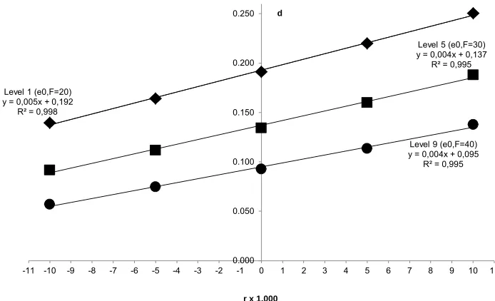
rate r different from zero and with crude death and birth rates stable over time). Figure 1 shows the relationship betweend and r for three levels of mortality in stable populations analyzed by C&D (West Family). At constant mortality levels, the value of
d changes according to the variation in r; in fact, if the birth rate is higher (or lower) than the death rate the proportion of infants increases (or decreases) and the proportion of child deaths varies accordingly (Ségui and Buchet 2013; Bocquet-Appel 2002; Masset and Bocquet 1977; Bocquet-Appel and Masset 1996). For example, in cases in which mortality is very high (such as level 1 C&D, e0,F = 20), where the population
increases annually by 1%, d = 0.250; conversely, if the population decreases by 1% thend = 0.139.
Figure 1: Relationship between d = (D5-19/D5+) and r, stable populations of
Coale & Demeny, West Family
These results raise doubts about the possibility of usingd directly as an indication of mortality level. Suppose that we only know the value of d = 0.137 for a single cemetery, without knowing the natural growth rate of the population. This value ofd
would be compatible with e0,F = 20 and r = –11‰, with e0,F = 30 and r = 0, and also
with e0,F = 40 and r = +11‰.
Level 1 (e0,F=20) y = 0,005x + 0,192
R² = 0,998
Level 5 (e0,F=30) y = 0,004x + 0,137
R² = 0,995
Level 9 (e0,F=40) y = 0,004x + 0,095
R² = 0,995
0.000 0.050 0.100 0.150 0.200 0.250
-11 -10 -9 -8 -7 -6 -5 -4 -3 -2 -1 0 1 2 3 4 5 6 7 8 9 10 11 d
However, if the annual population growth rate is low, then the influence of r over
d is quite limited; for example, again in the case of high mortality (level 1 C&D, e0,F = 20), if r varies within the interval ±3‰ then 0,177<d<0,207. More generally, as
pointed out by Figure 1, if r varies in the range of ±3‰, as in the case of stable populations, thed index offers a direct measure of the level of mortality. In addition, Figure 1 shows that the relationship between r andd is sufficiently linear and regular for mortality levels typical of pre-industrial societies (e0<40). Therefore, on the basis of
the empirical relationships visible in Figure 1, it is possible to correctd:
d* =d – 0,0045r wherer is expressed in ‰ and the coefficient of 0.0045 is the average of the slope coefficients of the lines in Figure 1.
Thed*index can be used to estimate the mortality level when the rate of natural growth r is known. For example, in a population where d = 0.250 and r = +10‰, then d* = 0.205, which corresponds to e0,F = 18.5 (and not e0,F<15, as would result when
usingd in a direct way).
Otherwise, in periods characterized by recurrent and intense mortality crises – such as in Italy in the three centuries between 1350 and 1650 and, in all likelihood, between the 6th and 7th centuries – the assumption of a stable population does not hold (Bocquet-Appel and Bacro 2008; Ségui at al. 2006; Signoli et al. 2002; Castex and Cartron 2007) because during the crises the number of deaths could increase five to tenfold compared to normal years, and also because the crises influenced other aspects of demography (Del Panta 1980). In particular, during periods of crisis the number of births might significantly decrease and many people might migrate to increase their chances of survival. Moreover, following a crisis marriages and births generally increased while mortality decreased, especially if the crisis had eliminated the weakest individuals.
To understand the meaning ofdin such circumstances, we performed a simulation. Starting with the female stationary population connected to mortality A of C&D level 1 Family West (e0,F = 20.0 and crude birth and mortality rate = 0.05), we hypothesized
In addition, in the simulation the birth rate is reduced by 40% in the year following the crisis, is increased in the following four-year period (+60% compared to a normal year), and then gradually approaches pre-crisis levels (+20% compared to the levels registered during the final five years). These trends are close to those in the parish of Nonantola (Modena) during the plague of 1630 (Alfani and Cohn 2007a). Therefore, in the three five-year cycles the birth rate is respectively 0.05 (to C&D level 1), 0.07, and 0.06.
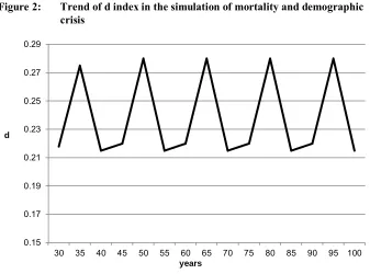
Under these hypotheses, the population fluctuates around the value observed at the beginning of the period (r=+0.35‰ over the century). Thirty years after the beginning of the crisis, d oscillates as shown in Figure 2, with an average level of 0.24 (life expectancy at birth slightly above 15 years) and a peak in the years of outbreak. Thus, the distribution of deaths among young adults and older people is close to that observed when the same life expectancy remains constant in time in a stationary population regime.
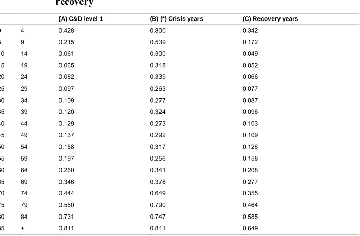
Table 1: Probability of dying in three five-year cycles of normality, crisis, and recovery
(A) C&D level 1 (B) (*) Crisis years (C) Recovery years 0 4 0.428 0.800 0.342
5 9 0.215 0.539 0.172 10 14 0.061 0.300 0.049 15 19 0.065 0.318 0.052 20 24 0.082 0.339 0.066 25 29 0.097 0.263 0.077 30 34 0.109 0.277 0.087 35 39 0.120 0.324 0.096 40 44 0.129 0.273 0.103 45 49 0.137 0.292 0.109 50 54 0.158 0.317 0.126 55 59 0.197 0.256 0.158 60 64 0.260 0.341 0.208 65 69 0.346 0.378 0.277 70 74 0.444 0.649 0.355 75 79 0.580 0.790 0.464 80 84 0.731 0.747 0.585 85 + 0.811 0.811 0.649
Figure 2: Trend of d index in the simulation of mortality and demographic crisis
Therefore, in periods afflicted by the coming and going of major epidemics, the value ofd may have been relatively high, corresponding to a kind of average mortality between years of very frequent epidemic outbreaks and years of normal mortality or recovery. If recovery was determined by an increase in the birth rate, thend could also be augmented by the high number of births.
Summarizing the calculations, observations, and simulations described above, it can be argued that the indicatord =15D5/D5+ is useful in estimating mortality when we
only have data on deaths derived from skeletal samples at our disposal, notwithstanding the limits of synthesizing an entire mortality regime by a single parameter. In the case of stationary populations or populations with a natural growth rate r between ±3‰, the indicator is well correlated to some basic parameters of mortality: asd grows, mortality increases. If r is larger or smaller, however, it is appropriate to correct the value ofd to take into account variations in the age structure of the population, and thus of deaths, due to the increasing or decreasing birthrate, according to the formula d* =d– 0.0045r‰, under the hypothesis that the C&D standard tables fit the mortality patterns well before the onset of the health revolution.
In general, sinced is influenced by the growth rate, it is inappropriate to use it to estimate mortality for a single cemetery or for a population of unknown trends over
0.15 0.17 0.19 0.21 0.23 0.25 0.27 0.29
30 35 40 45 50 55 60 65 70 75 80 85 90 95 100
d
time. On the contrary – as in the example shown below – the index is most useful when observed in a large number of cemeteries (or in any case referring to data on deaths related to several populations) so that the impact of anomalies – frequent in past populations – is diluted, and when population trends are known. Less problematic is the use of d to estimate the mortality of populations characterized by sudden dips and subsequent recoveries. In fact, in the long run, in these cases d is associated with measures of mortality in a manner not very different to those detected in stationary or stable population, although it may be also influenced by a higher proportion of young people. However, ifd can be a reliable estimator of mortality after the fifth birthday, caution is needed when estimating overall mortality, which could be greatly affected by the relatively abnormal mortality of children. Finally, under some reasonable hypotheses, the index d can also be used to detect different mortality patterns among males and females in societies of the past (Barbiera, Castiglioni, and Dalla-Zuanna 2016b).
3. The trends of d and the Italian population across the centuries
Starting from a previous study of the trends of d and its relationship to variations in mortality from Roman times to the end of the 12th century (Barbiera and Dalla-Zuanna
2007, 2009), we extended the data collection and the estimation of d to a later period running from the 13th to the 15th century. We considered only cemeteries with more
than 40 individuals, excluding those where more than 20% of adult skeletons were of unknown sex or age. In addition, we included only sites having a finald value between 0.15 and 0.30. Thus, out of hundreds of cemeteries found in the literature, we selected data from 43 sites comprising 4,244 individuals over five years of age (Barbiera, Castiglioni, and Dalla-Zuanna 2016c).
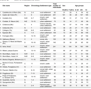
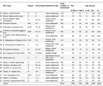
One important issue is that of chronology. Since most of the cemeteries were in use over long chronological spans and the graves and the bones they contained were very rarely dated with precision, it is not easy to use such data to illustrate changes over time. Hence, we decided to adopt the method proposed by Steckel (2010), which consists of grouping individuals buried within a given time span and assuming that the burials are evenly distributed across the dates in which the sites were in use. We then organized the results by century, thus estimating a mean number of skeletons aged 5–19 years and over 20 years of age for each century considered. For instance, 4 individuals aged 5–19 and 36 individuals over 20 years of age were identified in the cemetery of Torcello, S. Fosca (see Table 2, n 39), which dates from the 10th to the 12th century. We
each century. We finally added together the individuals thus estimated for each century and estimated the value of d for each 100-year time span. In this way, the obtained values are indicative of more general trends.3
Table 2: List of considered sites
Site name Region Chronology Settlement type Total number of individuals
Sex Age groups
M (20+) F (20+) 5–19 20+ 5+ 1 Castellecchio di Reno (Bo) N 2–4 rural settlement 62 31 20 8 54 62 2 Castro dei Volsci (Fr) C 6 rural settlement 201 101 56 28 157 185 3 Centallo (Cn) N-W 6–7 church, rural
settlement 162 66 31 27 114 141 4 Cividale, S. Mauro (Ud) N-E 13–15 urban settlement 72 33 14 17 49 66 5 Civitanova (Mc) C 4 Colonia Claudia,
urban settlement 181 62 57 19 119 138 6 Collecchio (Pr) N 7 rural settlement 154 36 25 27 77 104 7 Collegno (To) N-W 6–8 rural settlement 81 38 16 18 54 72 8 Egnazia (Br) S 1–4 urban settlement 136 13 28 18 88 106 9 Formigine (Mo) N 13–15 church, ruralsettlement 147 35 29 37 67 104 10 Gallicano (Roma) C 4 roman villa 105 36 32 18 68 86 11 Gerace, S. Maria del Mastro(Rc) S 15–18 church, urbansettlement 145 35 30 25 65 90
12 Iskra, Kranj* N-E 6–11 church, urbansettlement 241 59 104 36 163 199
13 Milano, piazza Duomo N 13–14 church, urban
settlement 104 60 27 15 87 102 14 Mont-Blanc, Aosta 1-2 N-W 2–5 rural settlement 133 45 46 17 91 108 15 Mont-Blanc, Aosta 3-4 N-W 6–8 rural settlement 131 40 34 12 74 86 16 Monte d’Argento, Minturno (Lt) C 11–15 church, urbansettlement 127 70 39 14 105 119
17 Monte di Croce, Pontassieve(Fi) C 11 church, castle 71 22 5 12 29 41 18 Ortaria, Povegliano (Vr) N 7 rural settlement 98 49 36 9 85 94 19 Pauciuri, Malvito (Cs) S 9–12 roman bath, urbansettlement 56 15 20 4 42 46 20 Poggibonsi (Si) C 7–13 rural settlement 41 22 16 9 38 47 21 Prata di Pordenone,S. Giovanni (Pn) N-E 13–15 church, ruralsettlement 62 34 9 7 47 54 22 Quadrella, Isernia S 1–4 rural settlement 99 26 28 8 54 62 23 Quingentole (Mn) N 7 rural settlement 70 26 18 15 58 73 24 Rimini C 2–4 Flaminia road,urban settlement 120 32 30 8 85 93
Table 2: (Continued)
Site name Region Chronology Settlement type Total number of individuals
Sex Age groups
M (20+) F (20+) 5–19 20+ 5+ 25 Roma, Casal Ferranti C 2 urban settlement 56 17 21 4 38 42 26 Roma, Osteria del Curato C 2 urban settlement 49 15 10 6 25 31 27 Roma, Palazzo dellacancelleria C 14–15 church urbansettlement 283 97 63 71 162 233 28 Romans d’Isonzo N-E 6–7 rural settlement 180 51 39 30 103 133 29 S Benigno Canavese (To) N-W 15–16 abbey, ruralsettlement 88 45 38 26 85 111
30 S Pietro di Cavallermaggiore(Cn) N-W 10–13 church, ruralsettlement 197 81 60 22 147 169 31 S. Agata, Piana degli Albanes(Pa) S 4–5 rural settlement 350 98 95 61 195 256 32 S. Sebastiano in Saluzzo (Cn) N-O 15 church, ruralsettlement 114 34 18 18 55 73
33 S. Vincenzino di Cecina (Li) C 5–8 roman villa, ruralsettlement 130 35 22 27 57 84
34 S.Lorenzo di Aversa S 10–12 Abbey, urbansettlement 49 28 8 5 40 45 35 San Caprasio Ad Aulla (Ms) N-O 9–15sec fortified village 79 32 23 10 63 73
36 Selvicciola (Vt) C 7 abandoned romanvilla, rural
settlement 110 49 20 16 73 89 37 Siena, S. Maria della Scala C 13–15 urban settlement 100 49 26 10 84 94 38 Torcello, cemetery (Ve) N 10–12 urban settlement 72 27 20 10 47 57 39 Torcello, S. Fosca (Ve) N 10–12 urban settlement 42 18 18 4 36 40 40 Trento, S. Virgilio (Ve) N 3–4 church, urbansettlement 175 73 64 14 137 151 41 Trino Vercellese (Vc) N-W 10–13 rural settlement 160 56 40 22 112 134 42 Urbino, S. Donato C 1–3 urban settlement 109 34 35 19 75 94 43 Vicenne, Campochiaro (Cb) S 7–8 rural settlement 76 28 24 5 52 57 Totals 5218 1853 1394 788 3456 4244
Note: * Iskra, Kranj is now Slovenia but was part of The Duchy of Friuli at the time it was in use.
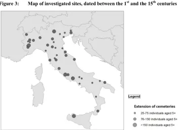
The individuals are generally evenly distributed across each chronological period considered and across the different Italian regions (Tables 2 and 3, Figure 3). However, it should be noted that for the Roman period we have a higher proportion of sites located in Southern-Central Italy, while for the medieval period more sites are available in the north. Furthermore, for some periods, such as the 1st, the 5th, and the 9th centuries,
only a few cemeteries satisfied our criteria, and for the 1st and the 9th centuries the
number of available individuals is low. Thus the results from data referring to these chronological spans might not be indicative of more general Italian trends. Moreover, between the 5th and the 8th centuries the percentage of skeletons from urban settlements
centuries of the early Middle Ages, graves were still few and were scattered within settlements. It is difficult for archeologists to identify them as they are often located under modern towns, and they were not taken into consideration in our study since they generally included less than 40 individuals. From the 9th century there was an increase
in burials in church buildings, so larger numbers of skeletons have been found and documented by archeologists (Barbiera 2015).
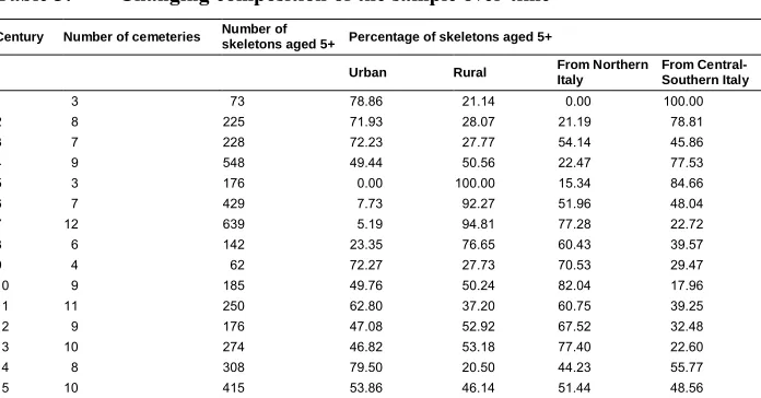
Table 3: Changing composition of the sample over time Century Number of cemeteries Number of
skeletons aged 5+ Percentage of skeletons aged 5+
Urban Rural From Northern Italy
From Central-Southern Italy 1 3 73 78.86 21.14 0.00 100.00 2 8 225 71.93 28.07 21.19 78.81 3 7 228 72.23 27.77 54.14 45.86 4 9 548 49.44 50.56 22.47 77.53 5 3 176 0.00 100.00 15.34 84.66 6 7 429 7.73 92.27 51.96 48.04 7 12 639 5.19 94.81 77.28 22.72 8 6 142 23.35 76.65 60.43 39.57 9 4 62 72.27 27.73 70.53 29.47 10 9 185 49.76 50.24 82.04 17.96 11 11 250 62.80 37.20 60.75 39.25 12 9 176 47.08 52.92 67.52 32.48 13 10 274 46.82 53.18 77.40 22.60 14 8 308 79.50 20.50 44.23 55.77 15 10 415 53.86 46.14 51.44 48.56
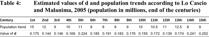
Keeping these points in mind, from our sample it emerges that the value ofd is relatively low between the 1st and 4th centuries, increases in the following period, when
the Justinianic Plague spread, and declines to a value similiar to that of Imperial Roman times between the 9th and the 13th centuries. By contrast, thed index is much higher in
those centuries after 1349 marked by the plague (Table 4). Hence, there is an increase indin periods characterized by mortality crisis.
Undoubtably, these data should be taken with caution because of all the problems inherent in using thed indicator as the only flag of mortality. For example, there may be conditions with very high infant mortality but low juvenile mortality, and vice versa. In that case thed indicator might underestimate (or overstate) the intensity of mortality: in the past the death of children under 5 years of age sometimes reached 50% of the total. Moreover, osteological data presents several problems. Even though for the purpose of this study we selected a sample of cemeteries that satisfy the above-mentioned criteria and which were extensively and accurately excavated (see Table 2 for details), nonetheless some problems should be borne in mind.
only 10%–20% of the total, while in the C&D standard table the percentages for those with an average age at death of 20 years, 30 years, and 40 years are 50%, 40%, and 25% respectively. This lack of children could be because they were buried separately from the adults, as demonstrated by several cemeteries found in different Italian regions and dated to different chronological periods where only children were buried (see Barbiera and Dalla-Zuanna 2007 for a discussion), or because the fragility of their bones resulted in their loss from the archeological record (Saunders et al. 2002). Employing thed ratio, as explained above, minimizes this shortcoming in the data.
On the other hand, it is difficult to identify selection by migration from the archeological record (Barbiera 2005). Seasonal migration may have meant that some individuals died in places that were not their habitual place of residence. Although traditionally considered a period of low population mobility, repopulation, depopulation, and colonization of virgin territories have also been documented for the Early Middle Ages (La Rocca 1992; Francovich 2002; Lazzari and Santos Salazar 2005). The Later Medieval Period (from the 10th–13th century) is even more
problematic, in that urbanization and the construction of new settlements likely had an impact on population mobility (Pinto 1996). Such phenomena, where intense and enduring, may have produced very specific distribution by age of population and thus also of deaths. To overcome this problem we considered cemeteries from various regions and from different settlements types, such as towns and villages (see Table 3). A final problem when dealing with a large territory such as the Italian peninsula is that different micro regions might have been characterized by different demographic patterns. Our research cannot detect diversity at such a detailed level because to date the number of sites at our disposal is quite limited. Given that this study includes almost all published data, perhaps this matter will be clarified when more skeletal data becomes available. At the present state of research we can reveal some general changes that characterize the different chronological periods, thus opening the path for future study.
Nonetheless, one positive point is that thed trend can be read together with the population trend (estimates of Lo Cascio and Malanima 2005): when d grows the population tends to decrease, and vice versa. An exception is the high value ofd in the 5th century, which might be distorted by the low number of cemeteries we have for this
Table 4: Estimated values of d and population trends according to Lo Cascio and Malanima, 2005 (population in millions, end of the centuries) Century 1st 2nd 3rd 4th 5th 6th 7th 8th 9th 10th 11th 12th 13th 14th 15th Population trend 15 12 9 10 11 8 8 8 9 10 10.5 11 12.5 8 9 Value ofd 0.175 0.144 0.146 0.169 0.224 0.185 0.191 0.183 0.176 0.155 0.172 0.139 0.174 0.241 0.252
When an epidemic appears the number of deaths rapidly increases to a peak and then begins to fall again. During the mortality crisis the number of marriages decreases drastically due to grieving and the disaggregation of kinship and social relations, the slowdown of economic and trade activities, and emigration to less affected areas. Thus, a sharp decline in conceptions and births follows, which, together with the deaths, decimates the population. The population, however, is extremely resilient and follows the typical Malthusian pattern. In fact, generally a year after the plague a strong recovery in weddings and births begins, which is due to a decline in the age at marriage, a reduction in those never married, and a shortening of the gap between births (Del Panta 1980; Livi Bacci 2000; Alfani and Cohn 2007b; Dalla-Zuanna et al. 2012; Green 2014).
For example, the parish baptism registers of the city of Florence indicate that in the 15thcentury the number of children baptized decreased by an average of 18% in the
years of plague and immediately afterwards. Subsequently, when the outbreak ended, the number of baptisms rose to higher levels than in the pre-plague years. So, for instance, during the outbreak of 1457 the number of children baptized was 1,882, in the preceeding years (1453–1456) it had been on average 2,113, while in the following years, between 1459 and 1461, the average number of baptisms was 2,123 (Herlihy and Klapisch-Zuber 1978). Written sources from the period report a strong increase in marriages and fertility following plague outbreaks: The population pyramid broadens, with a larger presence of children, who, once they reach adulthood, will contribute even more to the growth of the population by marrying at young ages and giving birth to many children. The population will therefore be young and vulnerable once again to new epidemics, since those who were immunized will have since died. In fact, it seems that the epidemic cycles of the years 1363/1364, 1374, 1383, and 1400 affected mainly children who were not immunized by previous outbreaks (Herlihy and Klapisch-Zuber 1978). The epidemic cycles at the end of the 15th century, which cyclically decimated
extraordinary numbers of children and the youth every ten years, considerably modified the age structure of the Italian population and compromised its chances of recovery. The high values ofd found for Italian cemeteries of this period represent these trends of mortality and recovery and selective mortality by age. In fact, because the increase ind
corresponds by extension to an increase in overall mortality) and an increase in births (and consequently an increase in young deaths, subsequently buried in the cemeteries) (Bocquet-Appel and Naji 2006; McCaa 2005). Our simulations described above do not contradict this interpretation.
4. Conclusions
Using the age-related indexd =15D5/D5+, estimated by cemetery, we were able to gather
information on the mortality regimes of both ‘normal’ population periods with moderate growth or decline and population periods affected by recurrent major epidemic cycles. In the latter, our simulation shows that d may be high because the mean level of mortality is higher than in periods without strong mortality crises and because the population is younger, as births exceed deaths in the years following the epidemic outbreaks.
It is hoped that this path of research will be extended, using the d index to investigate different geographical areas and chronological periods. Regarding our specific example of Italy during the first 1,500 years A.D., archaeological data should be implemented to provide newly excavated and analyzed osteological data, particularly for the early modern period; in this way it will be possible to appreciate regional differences and to systematically compare mortality trends obtained from skeletal samples with the data from cadasters, allowing reconstruction of the age structure of the population (although underestimation of children is sometimes evident in these cases also) in different areas and historical moments (Dalla-Zuanna et al. 2012). This comparison could be broadened to include mortality data collected in the first parochial registers.
5. Acknowledgments
The authors wish to profoundly thank Lorenzo Del Panta, Guido Alfani, the
References
Alfani, G. and Cohn, jr., S.K. (2007a). Nonantola 1630: Anatomia di una pestilenza e meccanismi del contagio.Popolazione e Storia 8(2): 99–138.
Alfani, G. and Cohn, jr., S.K. (2007b). Households and plague in Early Modern Italy.
The Journal of Interdisciplinary History 38(2): 177–205. doi:10.1162/jinh. 2007.38.2.177.
Alfani, G. and Bonetti, M. (in press). A survival analyses of the last great European plagues: The case of Nonantola (northern Italy) in 1630.Population Studies. Barbiera, I. (2005). Changing lands in changing memories: Migration and identity
during the Lombard Invasions. Florence: All’Insegna del Giglio.
Barbiera, I. (2015). Buried together, buried alone: Christian commemoration and kinship in the early Middle Ages. Early Medieval Europe 23(4): 385–409.
doi:10.1111/emed.12118.
Barbiera, I. and Dalla-Zuanna, G. (2007). Le dinamiche della popolazione nell'Italia medievale. Nuovi riscontri su documenti e reperti archeologici. Archeologia Medievale 34: 19–42.
Barbiera, I. and Dalla-Zuanna, G. (2009). Population dynamics in Middle Ages Italy before the Black Death of 1348: New discoveries from archaeological findings.
Population and Development Review 35(2): 367–389. doi:10.1111/j.1728-4457.2009.00283.x.
Barbiera, I., Castiglioni, M., and Dalla-Zuanna, G. (2016a). Why paleodemography? In: Matthijs, K., Hin, S., Matsuo, H., and Kok, J. (eds.). The future of historical demography: Upside down and inside out. Den Haag: Acco Publishers: 22–27. Barbiera, I., Castiglioni, M., and Dalla-Zuanna, G. (2016b). Missing women in the
Italian middle ages? Data and interpretation. In: Huebner, S. and Nathan, G. (eds.). The ‘Mediterranean family’ from antiquity to the Early Modern period: Proceedings of the International Conference at the Max-Planck Institute for Demographic Research, Rostock, June 14/15, 2012. Oxford: Wiley: 283–309.
doi:10.1002/9781119143734.ch15.
Bocquet-Appel, J.-P. (2002). Paleoanthropological traces of a Neolithic demographic transition.Current Anthropology43(4): 637–650.doi:10.1086/342429.
Bocquet-Appel, J.-P. and Masset, C. (1982). Farewell to paleodemography. Journal of Human Evolution 11(4): 321–333.doi:10.1016/S0047-2484(82)80023-7. Bocquet-Appel, J.-P. and Masset, C. (1996). Paleodemography: Expectancy and false
hope.American Journal of Physical Anthropology 99(4): 571–583.doi:10.1002/ (SICI)1096-8644(199604)99:4<571::AID-AJPA4>3.0.CO;2-X.
Bocquet-Appel, J.-P. and Naji, S. (2006). Testing the hypothesis of a worldwide Neolithic demographic transition: Corroboration from American cemeteries.
Current Anthropology 47(2): 341–366.doi:10.1086/498948.
Bocquet-Appel, J.-P. and Bacro, J.-N. (2008). Recent advances in paleodemography: Data, techniques, patterns. Dordrecht: Springer. doi:10.1007/978-1-4020-6424-1.
Castex, D. and Cartron, I. (2007).Epidémies et crises de mortalité du passé. Bordeaux: Ausonius Editions.
Coale, A. and Demeny, P. (1983). Regional model life tables and stable population. New York: Academic Press.
Dalla-Zuanna, G., Di Tullio, M., Leverotti, F., and Rossi, F. (2012). Population and family in central and northern Italy at the dawn of the Modern Age: A comparison of fiscal data from three different areas. Journal of Family History
37(3): 284–302.doi:10.1177/0363199012439007.
Del Panta, L. (1980).Le epidemie della storia demografica italiana (secoli XIV–XIX). Turin: Loescher.
Francovich, R. (2002). Changing structures of settlements. In: La Rocca, C. (ed.).Italy in the Early Middle Ages. Oxford: Oxford University Press: 144–167.
Galofré-Vilà, G., Hinde, A., and Guntupalli, A. (2017). Heights across the last 2000 years in England. Oxford: University of Oxford (Discussion Papers in Economic and Social History 151).
Green, M.H. (2014). Taking pandemic seriously: Making the Black Death global. In: Green, M.H. (ed.). Pandemic diseases in the medieval world: Rethinking the Black Death. Kalamazoo and Bradford: ARC Medieval Press: 27–62.
Hollingsworth, M.F. and Hollingsworth, T.H. (1971). Plague mortality rate by age and sex in the parish of St. Botolph’s without Bishopgate, London, 1603.Population Studies 25(1): 131–146.doi:10.1080/00324728.1971.10405789.
Hoppa, D.R. (2002). Paleodemography: Looking back and thinking ahead. In: Hoppa, D.R. and Vaupel, J.W. (eds.). Paleodemography: Age distributions fom skeletal samples. Cambridge: Cambridge University Press: 9–28. doi:10.1017/CBO 9780511542428.
Hoppa, R.D. and Vaupel, J.W. (2002). Paleodemography: Age distribution from skeletal samples. Cambridge: Cambridge University Press. doi:10.1017/CBO 9780511542428.
Koepke, N. and Baten, J. (2005). The biological standards of living in Europe during the last two millennia. European Review of Economic History 9(1): 61–95.
doi:10.1017/S1361491604001388.
La Rocca, C. (1992). Le necropoli altomedievali, continuità e discontinuità: Alcune riflessioni. In: Brogiolo, G.P. and Castelletti, L. (eds.). Il territorio tra tardoantico e altomedioevo: Metodi di indagine e risultati:Terzo seminario sul tardo antico e l’alto medioevo nell’Italia alpina e padana (Monte Barro, Galbiate, settembre, 1991). Florence: All’Insegna del Giglio: 21–29.
Lazzari, T. and Santos Salazar, I. (2005). La organización territorial en Emilia en la transición de la Tardoantigüedad a la Alta Edad Media (siglos VI–X). Studia Historica: Historia Medieval23: 15–42.
Leverotti, F. (1982). Massa di Lunigiana alla fine del Trecento: Ambiente, insediamenti, paesaggio. Pisa: Pacini.
Livi Bacci, M. (2000). Mortality crisis in historical perspective: The European experience. In: Corina, G.A. and Paniccià, R. (eds.). The mortality crisis in transitional economies. Oxford: Oxford University Press: 38–58.
Lo Cascio, E. and Malanima, P. (2005). Cycles and stability: Italian population before the demographic transition (225 B.C. – A.D. 1900).Rivista di Storia Economica
21(3): 5–40.
Masset, C. and Bocquet, J.-P. (1977). Estimateurs en paléodémographie. L’Homme
McCaa, R. (2005). Paleodemography of the Americas from ancient times to colonialism and beyond. In: Steckel, R.H. and Rose, J.C. (eds.). The backbone of history: Health and nutrition in the Western hemisphere. Cambridge: Cambridge University Press: 94–124.
Pinto, G. (1996). Dalla tarda antichità alla metà del XVI secolo. In: Del Panta, L., Livi Bacci, M., Pinto, G., and Sonnino, E. (eds.). La popolazione italiana dal medioevo a oggi.Bari: Leterza: 15–71.
Santini, A. and Del Panta, L. (1982).Problemi di analisi delle popolazioni del passato in assenza di dati completi. Bologna: Cleub.
Saunders, S.R., Herring, A., Sawchuk, L., Boyce, G., Hoppa, R., and Klepp, S. (2002). The health of the middle class: The St. Thomas’ Anglican Church cemetery project. In: Steckel, R.H. and Rose, J.C. (eds.).The backbone of history: Health and nutrition in the Western hemisphere. Cambridge: Cambridge University Press: 130–161.doi:10.1017/CBO9780511549953.007.
Ségui, I. and Buchet, L. (2013). Handbook of paleodemography. Cham: Springer.
doi:10.1007/978-3-319-01553-8.
Ségui, I., Pennec, T., Tzortyis, S., and Signoli, M. (2006). Modélisation de l’impact dèmographique de la peste à travers l’exemple de Maryigues (Buches du Rhône). In: Buchet, L., Dauphin, C., and Ségui, I. (eds.).La paléodémographie. Mémorie d’os, mémorie d’hommes. Antibes: APDCA: 323–330.
Scheidel, W. (2001). Progress and problems in Roman demography. In: Scheidel, W. (ed.).Debating Roman demography. Leiden: Brill: 1–81.
Signoli, M., Ségui, I., Biraben, J.-N., and Dutour, O. (2002). Paleodemography and historical demography in the context of an epidemic: Plague in Provence in the eighteenth century.Population57(6): 821–847.doi:10.3917/pope.206.0829. Steckel, R.H. (2010). The Little Ice Age and health: Europe from the early Middle Ages
to the nineteenth century [unpublished manuscript]. Columbus: Ohio State University.