Volume 62, 2019, Pages 78–91
SUMO User Conference 2019
Low-dimensional estimation and prediction
framework for description of the oscillatory
traffic dynamics
Jakub Krol
1,∗, Bani Anvari
1,∗, and Roberto Lot
2∗
Corresponding authors
1
Centre for Transport Studies, Faculty of Engineering, University College London, WC1E 6BT, UK
2
Faculty of Engineering and the Environment, University of Southampton, SO17 1BJ, UK
[email protected] [email protected] [email protected]
Abstract
Large majority of control methodologies used in traffic applications require short-time prediction of the environment. For instance, in widely-used Model Predictive Control [1] employed to reduce fuel and energy consumption of vehicles in a platoon, information about future velocity profiles of leading vehicles is necessary. In such case, the dynamic model should provide information more detailed than prediction of averaged and global quantities. Additionally, if the control input is to be applied at high-frequencies, traffic model must be solved in a short period of time.
We propose a novel framework which addresses aforementioned problems by estimating the vehicle velocity at any location in the domain based on the real-time information from induction loops downstream. Additionally, our formulation is linear and low-dimensional (i.e. consists of few degrees of freedom) meaning that the estimation can be executed at high frequencies. First a mapping is constructed from velocities at discrete locations to the smooth continuous field, which is subsequently projected onto its most significant principal components. Next, current state of such system is estimated using Kalman filter by combining the linear, wave-like dynamics of the traffic with the instantaneous information provided by induction loops. Short-term traffic prediction is then achieved by integration of the model forward in time.
The proxy methodology is validated using SUMO simulation on the test case of the vehicles approaching a traffic junction. The performance is evaluated based on sampling reconstructed continuous waveform at the locations and timestamps of the vehicles in the reference data and calculating velocity errors. Separate cases are considered where drivers follow Intelligent Driver Model perfectly and with varying levels of uncertainty.
1
Introduction
methodologies can be in general categorised based on the frame of reference relative to the driver or to the side of the road. In the first case, models are largely based on the car following models and deal with platoon dynamics. The latter case aims to describe traffic using quantities such as density and flow, and models inspired by fluid dynamics. The reconciliation of both is non-trivial. Some attempts in this regards are summarised and compared in [5].
Traffic data can be collected through various methods (e.g., loop detectors, GPS) with various spatio-temporal granularity. In traffic data analysis, one of the challenges is to map traffic data collected from stationary detectors to a continuous field. In scientific investiga-tions, isotropic smoothing and anisotropic kernel-based smoothing are common approaches for processing and reconstructing velocity data collected from stationary detectors. Treiber and Helbing [6] proposed a kernel-based traffic-adaptive smoothing method to produce a detailed reconstruction of traffic conditions between stationary loop detectors, and to combine different data sources. Various studied demonstrated that a kernel-based interpolation is an accurate and robust approach in comparison to isotropic data smoothing methodologies [6, 7,8,9,10]. Another challenge in traffic data analysis is to decompose the high-dimensional traffic data into principal variables that approximate different classes of traffic. Principal Component Analysis (PCA) [11, 12] is commonly used for traffic matrix analysis [13, 14, 15,16]. Previous studies have shown that PCA can provide a good approximation of traffic classes with few principle components, however, its accuracy and efficiency decreases in the presence of large anomalies in the system [16,17].
In this paper, we propose a proxy method which estimates full velocity field based on induction loop measurements and subsequently uses wave-like dynamics for velocity prediction. In the first step continuous data is constructed using weighted average of vehicles present in the link. The dimension of resulting data is dependent on the discretisation level set by the user, and can lead to high-dimensional data. Low-dimensional state is constructed by a projection of continuous velocity-density field onto few principle components. Subsequently, an estimation using the Kalman filter is performed.
The paper is organized as follows: Sections 2 and 3 explain the proposed methodology and the case study in-details. The results of the proposed framework on the case studies are presented in Section4. The conclusions are summarised in Section5.
2
Problem Formulation
Fixed point sensors such as inductive loop detectors allow collecting speed data at constant spatial locations. In order to construct a velocity field based on real-time traffic measurements from inductive loops, we analyse the system using an Eulerian reference frame. The network is therefore discretised into a series of spatial locations with the objective of estimating velocity at each grid point. Given such an estimated state, a model is constructed to dynamically predict the evolution of the high-dimensional velocity field forward in time.
In order to achieve this objective, state-space formulation of the dynamical system is utilised
at+1=A(at), (1a)
yt=C(at). (1b)
of the system. In traffic modelling those can represent some measurements corresponding to a vehicle driving through the network or information from induction loops such as mean speed or flow. In this study,ytis a function of velocity measurements from induction loops at time
t. The functionA:Rr→Rrdescribes dynamics of the system, whilstC:Rr→Rpis mapping between state and observations. The broad aim of the proposed estimation methodology is to infer current stateat given, usually imperfect, forms ofyt, A, C.
The estimation framework is constructed using the following steps:
• Constructing continuous velocity fields on the analysed network from discrete measure-ments associated with vehicles in the system (see Section2.1).
• Reducing the number of degrees of freedom by projecting data onto low-dimensional vector space in order to make the problem tractable for larger networks (see Section2.2).
• Defining a linear dynamic model on the low-dimensional state together with linear map between the state. Subsequently, combining both models together through a Kalman filter (see Section2.3).
Detailed description of each step is given in the following subsections.
2.1
Construction of a continuous velocity field
The availability of a continuous form of the velocity field allows us to assign the speed at any point in the domain for a certain prediction horizon and consequently reconstruct future velocity profile of a vehicle. Nonetheless, traffic data is given in the discrete form, where vehicles speed is associated with only one spatial location. In order to map discrete measurements into continuous domain we use modified Adaptive Smoothing Method (ASM) [6].
For a given link at timetj, there existn(tj)∈Nmeasurementszi,j=z(xi, tj) representing a characteristic quantity and acquired at irregular locationsxi fori≤n(tj). For example, they can be obtained using induction loops, wherezi,j could denote average velocity or flow. In the analysed case, zi,j represent instantaneous velocity of the vehicles in the system. Note that
n(tj) is not time-invariant and depends on the number of vehicles on the lane at each instance. The ASM mapszi,jto a regular grid space using the weighted average of the measurements close to each grid point such that
z(x, t) = 1
Pn(tj) i=1
Pjmax
j=jminΦ(∆x,∆t
∗)
n(tj)
X
i=1 jmax
X
j=jmin
Φ(∆x,∆t∗)zi,j, (2)
where weights are generated by a nonlinear kernel Φ(∆x,∆t∗), the appropriate form of which will be discussed later. The values of ∆x = xi−x and ∆t∗(c) = tj −t− ∆xc correspond respectively to spatial and temporal distances of measurement zi,j at xi, tj from grid point at x, t. Note that ∆t∗ depends on speed c which defines a rate at which measurements are propagated in the spatio-temporal domain. The ASM is based on the assumption that a traffic perturbation will either propagate downstream at free flow speedcf reeor upstream at congested speed ccong. Consequently, two interpolated quantities are obtained zf ree(x, t) for ∆t∗(cf ree) andzcong(x, t) for ∆t∗(ccong).
The final interpolated value zinterpis calculated as
Parameter Description Assigned Value (kmh )
cf ree Propagation velocity of perturbations in free traffic 80
ccong Propagation velocity of perturbations in congested traffic -15
Vc Crossover from free to congested traffic 60
∆V Width of the transition region 20
Table 1: A summary of the parameters and their typical values in the Adaptive Smoothing Method as defined in [6].
Here, the weightw(Vcong, Vf ree) is a function of smoothed velocities, i.e. Vf ree =zf ree ifzi,j denote speed measurement (with equivalent definition ofVcong), and is given by
w(Vcong, Vf ree) = 1 2
1 + tanh V
c−min(Vcong, Vf ree) ∆V
,
whereVcand ∆V are re-scaling parameters. Note when ∆V →0,w→1/2 such thatVcong and
Vf ree have equal weighting. Table1shows a summary of the values assigned to the parameters in the ASM in [6]. It is noted that the methodology is robust with respect to small changes in those parameters [6].
The final mapped quantity heavily depends on the choice of kernel Φ(∆x,∆t∗). In [6],
Φ(∆x,∆t∗) = exp
−|∆σx|−|∆t
∗|
τ
(3)
is used for spatial and temporal smoothing parameters σ andτ. In this study, the smoothed velocity field should take the same value aszi,j whenx=xi andt=tj, i.e.
lim
∆x→0,∆t∗→0Φ(∆x,∆t ∗)
→ ∞.
This is not the case in (3) and consequently the exponential kernel is replaced with
Φ(∆x,∆t∗) =
|∆x|2
σ +
|∆t∗|2
τ −1
. (4)
The relative decay of measurements in space and time can be regulated through appropriate choice of the smoothing parametersσ and τ. In the following analysis σ =τ = 1, however, further investigation is required to determine what values are the most beneficial for dynamic modelling purposes.
Note that Φ = 0 only when either ∆x → ∞ or ∆t → ∞. Here, the modified ASM is applied separately for each edge and consequently if vehicle is outisde of the spatial domain of interest, it is automatically assigned Φ = 0. Furthermore, note that temporal summation in (2) is bounded by hard limitsjminandjmax thus ignoringzi,j corresponding to large values of ∆t∗.
2.2
Dimensional reduction
Nonetheless, in a network with multiple links, the dimension of the problem can be too large for real-time applications and it is necessary to reduce the number of degrees of freedom.
The velocity field u(x, t) is therefore defined as a sum of time-invariant structures Φi(x) such that
u(x, t)≈u¯(x) + r X
i=1
ai(t)Φi(x), (5)
where the scalar coefficientai(t) is associated withΦi(x) and describes its evolution in time. The term ¯u(x) is a time-constant part of the dynamics and can represent, for example, mean flow or steady-state solution to the underlying equations. Given (5), in order to reduce the dimension of the problem,ai is set to be variables in state vector a. Note that now the sizer ofa∈Rr can be set freely allowing for drastic dimensional reduction.
There exists a large variety of possible choices for Φi(x) [18]. In the following analysis, Φi(x) will be set to the output of Principal Component Analysis (PCA) [11]. The PCA is a widely used technique which produces structuresΦi(x) that give the optimal approximation of (5) with respect tol2-norm and which are orthonormal (i.e. Φ
i(x)>Φj(x) =δijwhereδijis the Kronecker delta). The orthonormality ofΦi(x) is beneficial as it allows us to obtain projection coefficientsai(t) in a straightforward manner whereai(t) =Φi(x)>u(x, t). Furthermore, prin-cipal components are ordered with respect to explained variance making it easy to select ther
most important structures.
2.3
Dynamic model and estimator
In order to obtain the velocity field in the network, live information about PCA projection coefficients ai(t) are necessary. This can be obtained using the Kalman filter [19], which is state-space model-based estimation technique. Given imperfect dynamic model and some noisy measurements, Kalman filter can produce a state estimate which is more accurate based on a single set of measurements or integration of the dynamic model.
The estimated dynamical system is expressed in thelinearstate space formulation such that
at+1=Aat (6a)
yt=Cat (6b)
whereat= [a0(t), . . . , ar(t)]>. Note that functions in (1) are replaced with matricesA∈Rr×r,
C ∈Rp×r. The Kalman filter works by recursively applying a two-step procedure: prediction andupdate. In the prediction step, the values at the next step are obtained by propagating a current state forward in time using dynamical model, i.e. by applying (6a). Subsequently, once a new measurement is available the predicted step is updated based on the difference between acquired and predicted measurements, i.e. yt−Cat.
The Kalman filter algorithm was originally formulated for linear state dynamics and obser-vation mappings (with nonlinear extensions such as Extended Kalman Filter [20] or Unscented Kalman Filter [21] developed later). Due to simplicity and low-computation cost, a linear form will be utilised here. The values of A and C are obtained using a solution to least squares problem on some training data, i.e.
A= arg min
A∗
X
t
||at+1=A∗at||2, (7a)
C= arg min
C∗
X
t
Length Minimum headway Acceleration ability Deceleration ability Maximum velocity
5.0 m 2.0 m 0.8 m/s2 4.5 m/s2 25 m/s
Table 2: Vehicle parameters used in the simulation of Test Case 1.
Furthermore, the accuracy of Kalman filter estimates increases if the relative inaccuracies in the dynamical model and observation mapping are provided through process and observation noise covariance matrices,QandRrespectively. Using the same training data as in (7),Qand
Rare defined as
Q=epe>p (8a)
R=eme>m (8b)
where
ep=
a1−Aa0 . . . aN−AaN−1
em=
y0−Ca0 . . . yN−CaN
andN is the size of the training data.
3
Case Studies - Cars approaching a traffic junction
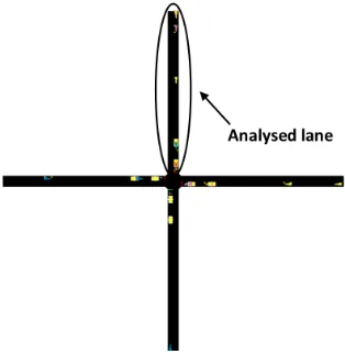
The methodology outlined in Section 2 is analysed on the simple test case of the vehicles approaching a junction on a link with single lane. The analysed scenario will be referred to as Test Case 1 and corresponding SUMO network is presented in Figure1. The investigated lane is 95.25m long and 3.20m wide. The induction loop is placed atx= 89.25m. The routes are generated such that the car enters the lane approximately every 10s leading to congested traffic conditions. First, it is assumed that each vehicles has identical parameters given in Table 2 and is driving according to Intelligent Driver Model (IDM) without any driver imperfections. Test Case 1 is simulated using SUMO 0.32.0 [22] fort≤2h. Data is sampled with the constant timestep ofδt= 0.1s, resulting in 72,000 sets of measurements.
In order to test the robustness of the estimation approach Test Case 2 is constructed which consists of multiple separate simulations. In this case, every vehicle is assigned with a certain degree of imperfection. For desired speed u∗(t) given by IDM, the speed of each vehicle is modified such that u(t) =ku∗(t). The value of k is chosen using the following procedure: 1) first,k is drawn from Gaussian distribution, k∼ N(1, σ2); 2) subsequently, in order to avoid excessively slow and fast vehicles in the network, lower and upper caps are introduced such that 0.2< k <2. Separate simulations are performed forσ2 =
{i∈N|i≤4}. It is noted that since the upper and lower caps are introduced, distribution ofk is no longer Gaussian and as
σ2→ ∞it will converge to Bernoulli distribution. Consequently,σ2does not describe variance ofkin a strict sense.
4
Results
Figure 1: Test case of vehicles approaching a junction is used to analyse the methodology presented in Section2.
4.1
Modified ASM analysis
The modified ASM methodology outlined in Section2.1is applied to data corresponding to all aforementioned Test Cases. The lane is discretised into 100 points and the temporal window in (2) is set such that jmax and jmin always satisfy jmax −jmin = 10s and t = 12(jmax+
jmin). The value of 10s is chosen so that weight Φ(0,∆t∗) generated using kernel (4) associated with measurements temporally furthest away satisfies Φ(0,∆t∗)<0.05. The spatio-temporal diagram of obtained from the modified ASM together with temporal and spatial snapshots at fixed locations are presented in Figure2.
(a)
0 50 100
Distance (
m
) 02 4
Sp
ee
d
(
m
/
s
)
(b)
100
Time (s)
200
0
2
4
6
Sp
ee
d (
m/
s)
(c)
Figure 2: (a) Spatio-temporal diagram obtained from the modified Adaptive Smoothing Method, (b) spatial snapshot at t = 200s, and (c) temporal snapshot at x = 48m. Note that locations of the snapshots are represented on the spatio-temporal diagram.
0 50 100 Distance (m) 0.08 0.10 Φ ( x )
Principal Component 1
(a)
0 50 100
Distance (m)
−0.1
0.0 0.1
Φ
(
x
)
Principal Component 2
(b)
0 50 100
Distance (m)
−0.1
0.0 0.1
Φ
(
x
)
Principal Component 3
(c)
100 200 300
Time (s) 0 10 20 30 a ( t )
Principal Component 1
(d)
100 200 300
Time (s) 0 20 a ( t )
Principal Component 2
(e)
100 200 300
Time (s) 0 20 a ( t )
Principal Component 3
(f)
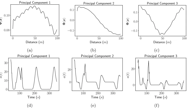
Figure 3: Three principal components of the data are presented in (a), (b) and (c), and their corresponding projection coefficients are illustrated in (d), (e) and (f) respectively.
whole length of the lane.
4.2
PCA analysis
Principal components of the data presented in Figure2are calculated in this section in order to obtain the separation of variable of the form (5). Note that, usually (5) contains a time-constant structure ¯u(x). However, here, ¯u(x) = 0 is chosen based on the assumption that if other form of ¯u(x) is significant, it will emerge asΦi(x) for which ˙ai(t)≈0.
The first three principal componentsΦi(x) and their corresponding projection coefficients
ai(t) are presented in Figure3. Although, principal component decomposition should be anal-ysed taking into account all components at the same time, a certain level of interpretation can be achieved by investigating each component individually. The shape of the first principal component in Figure3ademonstrates that the maximum velocity in the link is achieved in the middle of the lane. The second principal component in Figure3bshows vehicles departing from the analysed lane in the situation where traffic light stage changes to green. When its projec-tion coefficient becomes negative in Figure3e, an increase in velocity downstream is observed. Subsequently, when its coefficient becomes positive, upstream velocity field increases implying that the vehicles in the back of the queue start to accelerate. It should be noted that projection coefficients exhibit progressively higher frequencies for higher orders of principal components, representing harmonics of the system.
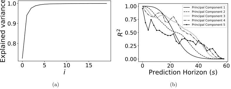
In order to choose the appropriate size of the low-dimensional space (rin (5)) singular values
si of the principal components are investigated. Singular values give us information regarding the explained varianceσ2
i of each principal component such that σ2i = s2i/ P
is 2
i. The total explained variance,σ2(r) =Pr
i=1σ 2
i as a function ofris analysed and presented in Figure4a. It can be seen that the value approaches σ2(r)
0 5 10 15
i
0.8 0.9 1.0
Ex
pl
ai
ne
d
va
ri
an
ce
(a)
0
20
40
60
Prediction Horizon (
s
)
0.00
0.25
0.50
0.75
1.00
R
2
Principal Component 1 Principal Component 2 Principal Component 3 Principal Component 4 Principal Component 5
(b)
Figure 4: (a) Shows the explained variances of the principal components corresponding to the data in2a, and (b) is theR2corresponding to linear model applied over a range of prediction horizons.
Consequently,r= 6 is chosen for further analysis.
4.3
Dynamical modelling
Linear model required in Kalman filter is obtained by solving (7a) on the training data set. Figure 4bshows the values of R2 for each of the projection coefficients when linear model is applied in order to predict state values over a range of future prediction horizonsth. It is showed that over a short period of time linear model provides a good description of the dynamics, where first four of the projection coefficients exhibitsR2 >0.6 forth>20s. It can be also seen that as the order of the projection coefficients increases the relationship betweenR2andt
hbecomes more irregular. This is due to the fact that PCA in many cases is able to separate noise and coherent structures into separate principal components, so that noise is primarily contained in higher order components. This feature is also visible in the analysed system where higher order projection coefficients contain high frequency oscillations.
In addition to dynamical model, it is necessary to provide measurements y which will be used to update statea. Using instantaneous velocity,u(t) from induction loop obtained directly from SUMO simulation, time-delayed valued are introduced in the construction ofysuch that
yt= [u(t), u(t−δt), . . . , u(t−nδt)]>forndelayed measurements. The mappingCis obtained by solving (7b). Noting that measurements are not available when there are no vehicles occupying the induction loop, (7b) is only solved fortwhenkytk0=n+ 1. The value ofnis chosen based on solution to the inverse problem
min
C−1 X
t
||C−1yt−at||2
and investigation of R2 corresponding to estimate of each state in a
t. It was observer that relative increase in value of R2 for n = 6 is less than 5% and consequentlyn = 5 is chosen. Despite omitting measurements whereytis not a full vector,N ≈30,000 samples are used to solve (7b).
100 200 300 Time (s) 0.0
2.5 5.0 7.5
a
(
t
)
Principal Component 1
Reference State Estimated State
(a)
100 200 300
Time (s) 0
5
a
(
t
)
Principal Component 2
Reference State Estimated State
(b)
100 200 300
Time (s) 0
10
a
(
t
)
Principal Component 3
Reference State Estimated State
(c)
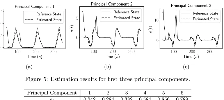
Figure 5: Estimation results for first three principal components.
Principal Component 1 2 3 4 5 6
i 0.242 0.284 0.382 0.584 0.856 0.789
Table 3: The relative squared errors (10) corresponding to results presented in Figure5.
4.4
Estimation results
4.4.1 Test Case 1
Using model obtained in Section 4.3 Kalman filter is applied to measurements y outside the training domain, covering initial portion of the data. Standard Kalman filter is modified to take into account the fact thaty is not available at every timestamp. Recalling that Kalman filter consists of prediction and update stages, here, when there are no vehicles occupying the induction loop only the prediction step is applied and the update stage is omitted. The estimated coefficients together with the reference data are presented in Figure5.
At the initial stage of the simulation vehicles enter the analysed domain for the first time, and the system is converging towards congested condition. The dynamics at that stage is highly nonlinear and such phenomena are not included in the training data. On the other hand for
t >150s, the system exhibits oscillatory wave-like behaviour, where the linear Kalman filter formulation provides accurate estimates. The relative squared error,
2i = P
t>150(ai(t)−ˆai(t)) 2
P
t>150(ai(t))2
(10)
is calculated for each of the estimated projection coefficients ˆaiwith the values shown in Table 3. It is observed that dynamics of the first three principal components is estimated accurately with i <0.5. The errors are larger for components of the higher order which correspond to frequencies higher than those which characterise the induction loop measurement. In those cases nonlinear mapping between state and measurement might be necessary. Nonetheless, it is noted that the contribution of the higher order components to explained variance is relatively small (see Figure4a) and the estimate errors should have significantly smaller impact on the accuracy of the reconstructed velocity field ˆu(x, t).
0 2 4 6 vi
0 2 4 6 8
̂ûx,ti
i
)
̂
ûxi, ti) = vi
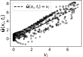
Figure 6: The scatter plot of velocitiesviand corresponding reconstructed velocity field ˆu(xi, ti).
1
2
3
4
σ
2
1
2
3
ε
iPrincipal Component 1 Principal Component 2 Principal Component 3 Principal Component 4 Principal Component 5
(a)i
1 2 3 4
σ
20.3 0.4 0.5
ε
v εRv20.7 0.8 0.9
R
2
(b)R2 and
h
Figure 7: The error metrics for estimation framework applied to data with imperfect drivers for a range ofσ2.
the error metric is given by
2v= P
i( ˆu(xi, ti)−vi)2 P
ivi2
. (11)
It is noted that the same vehicle is used multiple times in the error calculation but for different values ofxi andti.
The scatter plot of velocities vi and corresponding reconstructed velocity field ˆu(xi, ti) for
t >150s is given in Figure 6. Note that, for the visualisation purposes, data in Figure6 was subsampled and only randomly chosen 10% of all datapoints are presented. It is shown that the on average estimated velocity is in the same range as the reference value. The values ofv andR2 associated with results in Figure6 are 0.286 and 0.907 respectively.
4.4.2 Test Case 2
i.e. error in estimation coefficientsi(10) and error against discrete measurementsv (11), are presented in Figure7. It is showed that the estimation of the first three projection coefficients is robust with respect to σ2. On the other hand, higher order estimates give error of
i > 1 forσ2>2. Such values of
i implies that estimate of the coefficients is on average worse than a constant model, and estimation of those dynamical features in fact reduces accuracy of the reconstructed velocity field. This phenomenon is reflected in the rapid decrease ofR2in Figure 7b.
5
Conclusions
The methodology which estimates velocity profiles based on the real-time information from in-duction loops was presented. The current implementation is linear and low-dimensional making the demonstrated approach suitable in situations where computational cost and simplicity are of high importance. The system was analysed on a simple problem of vehicles approaching the traffic junction in a congested traffic. Such a system exhibits semi-linear dynamics and can be well estimated using projection onto few structures and linear formulation of Kalman filter. Additionally, model calculated based on a perfect data was applied to dynamics with driver imperfections, where the estimation of key dynamical features corresponding to first few principal components was showed to be robust.
The future work will involve the application of the developed methodology to more realistic test cases; first with smaller and variable levels of congestion and second with traffic perturba-tions. In those cases non-linear effects are expected to be of significance and will need to be implemented in the dynamical model (1). The exact form of nonlinearity will be either obtained from detailed analysis of car-following models or from data-driven model inference techniques. Additionally, the network level test case will be developed and examined, because it is believed that proposed technique is more suitable in systems with multiple road link since it allows for radical reduction of degrees of freedom.
Acknowledgement
This research is funded by the Engineering and Physical Sciences Research Council (EPSRC) [grant No.: EP/N022262/1] whose support is gratefully acknowledged. The authors also express appreciation to the SUMO community for the development and maintenance of the SUMO micro-simulation software package, and to Craig Rafter from the University of Southampton for his assistance and support to get familiar with SUMO.
References
[1] Carlos E. Garcia, David M. Prett, and Manfred Morari. Model predictive control: theory and practice—a survey.Automatica, 25(3):335–348, 1989.
[2] Mark S. Young, Stewart A. Birrell, and Neville A. Stanton. Safe driving in a green world: A review of driver performance benchmarks and technologies to support ‘smart’driving. Applied ergonomics, 42(4):533–539, 2011.
[4] Rich C. McIlroy, Neville A. Stanton, and Catherine Harvey. Getting drivers to do the right thing: a review of the potential for safely reducing energy consumption through design. IET Intelligent Transport Systems, 8(4):388–397, 2013.
[5] Eleni I. Vlahogianni, Matthew G. Karlaftis, and John C. Golias. Short-term traffic forecasting: Where we are and where we’re going. Transportation Research Part C: Emerging Technologies, 43:3–19, 2014.
[6] Martin Treiber and Dirk Helbing. An adaptive smoothing method for traffic state identification from incomplete information. InInterface and Transport Dynamics, pages 343–360. Springer, 2003. [7] J.W.C. Van Lint and Serge P. Hoogendoorn. A robust and efficient method for fusing heteroge-neous data from traffic sensors on freeways.Computer-Aided Civil and Infrastructure Engineering, 25(8):596–612, 2010.
[8] Martin Treiber, Arne Kesting, and R. Eddie Wilson. Reconstructing the traffic state by fusion of heterogeneous data. Computer-Aided Civil and Infrastructure Engineering, 26(6):408–419, 2011. [9] Felix Rempe, Philipp Franeck, Ulrich Fastenrath, and Klaus Bogenberger. Online freeway traffic
estimation with real floating car data. In2016 IEEE 19th International Conference on Intelligent Transportation Systems (ITSC), pages 1838–1843. IEEE, 2016.
[10] Zhoutong Jiang, Xiqun Michael Chen, and Yanfeng Ouyang. Traffic state and emission estimation for urban expressways based on heterogeneous data. Transportation Research Part D: Transport and Environment, 53:440–453, 2017.
[11] Ian Jolliffe. Principal component analysis. In International encyclopedia of statistical science, pages 1094–1096. Springer, 2011.
[12] Michael E. Tipping and Christopher M. Bishop. Probabilistic principal component analysis. Jour-nal of the Royal Statistical Society: Series B (Statistical Methodology), 61(3):611–622, 1999. [13] Theodore Tsekeris and Antony Stathopoulos. Measuring variability in urban traffic flow by use of
principal component analysis.Journal of Transportation and Statistics, 9(1):49, 2006.
[14] Qu Li, Hu Jianming, and Zhang Yi. A flow volumes data compression approach for traffic net-work based on principal component analysis. In 2007 IEEE Intelligent Transportation Systems Conference, pages 125–130. IEEE, 2007.
[15] Xuexiang Jin, Yi Zhang, Li Li, and Jianming Hu. Robust pca-based abnormal traffic flow pattern isolation and loop detector fault detection. Tsinghua Science & Technology, 13(6):829–835, 2008. [16] Xingxing Xing, Xiabing Zhou, Haikun Hong, Wenhao Huang, Kaigui Bian, and Kunqing Xie. Traf-fic flow decomposition and prediction based on robust principal component analysis. In2015 IEEE 18th International Conference on Intelligent Transportation Systems, pages 2219–2224. IEEE, 2015.
[17] Chenyi Chen, Yin Wang, Li Li, Jianming Hu, and Zuo Zhang. The retrieval of intra-day trend and its influence on traffic prediction. Transportation research part C: emerging technologies, 22:103–118, 2012.
[18] Laurens Van Der Maaten, Eric Postma, and Jaap Van den Herik. Dimensionality reduction: a comparative review. J Mach Learn Res, 10:66–71, 2009.
[19] Rudolph Emil Kalman. A new approach to linear filtering and prediction problems. Journal of Basic Engineering, 82(1):35–45, 1960.
[20] Harold W/ Sorenson and Allen R. Stubberbud. Non-linear filtering by approximation of the a posteriori density. International Journal of Control, 8(1):33–51, 1968.
[21] Eric A. Wan and Rudolph Van Der Merwe. The unscented kalman filter for nonlinear estimation. InAdaptive Systems for Signal Processing, Communications, and Control Symposium 2000. AS-SPCC. The IEEE 2000, pages 153–158. Ieee, 2000.