A Tool for Daily Demand Pattern Generation

A Tool for Daily Demand Pattern Generation

Gargano R.

_{, Tricarico C.}

_{, Santopietro S.}

_{, de Marinis G.}

_{, Silvagni G.}

2 _{Università degli Studi di Roma Torvergata, via del Politecnico 1- 00133 Roma, Italy}

gargano@unicas.it, c.tricarico@unicas.it, s.santopietro@unicas.it, demarinis@unicas.it,

silvagni@ing.uniroma2.it

Abstract

A correct water demand characterization is at the base of a reliable water distribution system simulation. The stochastic nature of water demand is well established and thus has to be addressed. In the present work a methodology to generate synthetic demand patterns interpolating known points by means of piecewise interpolation has been implemented in Python. Subsequently a stochastic approach has been applied to the interpolated demand patterns, which is based on a mixed probability distribution. Such approach considers the dual nature of water demand as continuous and discrete random variable, in order to contemplate both the event of it being null and not null. The needed parameters are obtainable through simple equations depending solely on the number of served users.

1

Introduction

Residential water demand characterization is one of the crucial aspects which still represents a great source of uncertainty in water distribution systems modelling.

In the last two decades many demand models have been proposed, and they either model the demand for end users or for clusters. In the first category there are some examples that have gained popularity like [1] that uses rectangular pulse models or [2] in which water demand variability is reproduced with CDF parameters that were estimated from experimental data.

The downside of this kind of models is that they are characterized by a difficult applicability due to the multiplicity of information they require for the parameters estimation. This often results in a difficulty in the application of such approaches in general conditions, making them very case specific. Indeed, the pursuit of a very fine detail in the demand characterization implies a very complex implementation that compromises the applicability of such approaches in non-scientific contexts.

Recently in [3] an approach based on a mixed distribution (contemplating both null and not null demand) has been proposed to model demand for clustered users. This approach considers water demand to be combination of a discrete and a continuous random variable, the discrete one is used to

Volume 3, 2018, Pages 746–754

model periods of non-null demand. Furthermore, the only required parameters to calibrate and implement the model, are the number of served users and the average demand coefficient pattern.

Unfortunately, in many situations, especially in newly to-be developed projects, even the basic information might be difficult to infer. Daily demand patterns are obtained with measurements that can be really high in costs or be impossible to perform a priori, before that the work is accomplished.

In this study a Python tool is developed in order to generate congruent synthetic average demand pattern at the node level, by means of a piecewise polynomial interpolation, without considering temporal correlation between different instants. Some literature relations are considered for the estimation of the fixed points along the daily pattern, like the peaks and the minimum night flow, and then an optimization algorithm is applied to infer the unknown ones.

Subsequently a stochastic approach is applied in order to generate congruent demand patterns for a specified number of days. The tool has the feature to read and write demand patterns directly in EPANET 2.0 [4] input files, giving the user the ability to quickly generate demand scenarios for any network provided in that file format.

2

Methodology

As it is well known, residential water demand follows daily trends according to the habits of the users connected to the WDS. These trends are characterized by a variable number of peaks (usually 2 or 3) that represent the moments of highest consumption, and by a very low plateau that is localized in the night hours which can have a variable length and represent the moment of minimum consumption. These in the design process can be considered known points, given that they represent the inputs of the design process. Indeed, many works in scientific literature have tackled and analysed specifically the afore mentioned aspects of the daily demand pattern and thus can provide a good starting point for their estimation.

Once these points are set, in this work a piecewise polynomial interpolation is performed by means of the Piecewise Cubic Hermite Interpolating Polynomials, in order to obtain a continuous and periodic curve to represent the daily average demand pattern which is the starting point to perform a stochastic generation.

Here a clarification is needed, indeed the average daily demand pattern is strongly dependent on the time resolution that is considered. The time averaging process smoothens the trend of the pattern, reducing the entity of the peaks and reducing the probability of having null consumption during the night hours. These aspects will be further discussed in the following sections, but for the sake of this study a time resolution with a time interval ∆𝑡 = 1𝑚𝑖𝑛 is considered.

For the sake of this study we consider the dimensionless water demand by means of the demand coefficient:

𝐶

(𝑡) =

𝜇_𝑄

(1)

where 𝜇𝑄 is the daily mean water demand, and Q(t) the value of water demand at the time t.

In this situation, namely the normalization of the water demand against its mean, it is easy to see that the integral of the demand coefficient over one day is equal to 1 as shown in Eq.(2).

∫ 𝐶

(𝑡)𝑑𝑡 = 1

2.1

The peak coefficient

As said earlier within the daily demand pattern, particular significance is attributed to the peak water demand, which is the maximum expected water flow generated for a particular set of users. We hereby consider the peak demand coefficient, which as is the dimensionless ratio between the peak water demand 𝑄𝑝 and the mean water demand 𝜇𝑄.

𝐶

=

𝜇𝑄

(3)

The peak demand coefficient is the most onerous among the ordinary working conditions and it is relevant in many engineering applications. In particular it is taken into account in both the design and rehabilitation processes of WDSs.

It is well established in scientific literature that the peak coefficient is dependent on the number of users that generate the flow, specifically it decreases as the number of users increases. Several expressions have been proposed over the years to describe this behavior, from the well-known proposed by [5] to the more recent [6] and [7] which have recalibrated the former relation considering a more extended and heterogeneous dataset.

In this work the equation proposed in [7] has been considered ad is hereinafter displayed.

𝜇

= 10𝑁

−0,2

₍₄₎

Where 𝜇𝐶𝑃 is the mean demand coefficient and 𝑁𝑈𝑠, the number of served users. The peak

coefficient is strongly influenced by the considered time resolution. The time averaging process smoothens the daily trend reducing the peaks entity and in [8] and [7] it is possible to find relations that allow to estimate the decay of the peak demand as the time interval increases.

In real WDSs usually the demand pattern presents more than one peak, but usually the minor ones are considered less important since they do not represent a particular stress to the system. Usually the number and distribution of the peaks is strongly dependent on the users habit and varies from Country to Country. In this work the minor peaks are expressed as a portion of the main peak, by means of a multiplier that is always smaller than 1.

2.2

The minimum night flow (MNF)

Another peculiarity of the daily demand pattern it is represented by the night flow. This element is particularly interesting in practical applications because in this condition the water demand is at the lowest point and the pressures in the network reach their maximum value. Such event causes usually an increase of the expected leakages, and that is why in many studies that face leakages estimation, consider these to be strongly related to MNF (e.g. [9], [10]).

This period occurs in the night hours where the consumption is expected to be very low. Farley and Trow [11] assert that a good estimate is between 2:00 and 4:00 a.m. even if it is reasonable to say that it is strongly dependant on the considered users, in fact cultural and work habits might affect the occurrence and the duration of this time span.

different Countries, allowing to estimate the probability of the null water demand from the number of supplied users.

In the present study, the MNF is considered to be constant and its value, along with the duration of the period is considered to be an input parameter.

Finally, another important point needed to preserve the periodicity of the daily demand trend is the value that the demand coefficient 𝐶𝐷 assumes at midnight. This translates in setting for two points, at

0:00 and at 24:00, the demand coefficient.

2.3

Interpolating curves

Let us consider the entire day divided in 𝑛 intervals so that

0: 00 = 𝑡

< 𝑡

< ⋯ < 𝑡

= 24: 00

(5)

Let {𝑓𝑖∶ 𝑖 = 1, 2, … , 𝑛} be a given set of monotone data values at the partition points (knots); that

is, we assume either 𝑓𝑖≦ 𝑓𝑖+1(𝑖 = 1, 2, … , 𝑛 − 1) or 𝑓𝑖≧ 𝑓𝑖+1(𝑖 = 1, 2, … , 𝑛 − 1). The aim is to obtain

a piecewise cubic function 𝑝(𝑡𝑖) so that

𝑝(𝑡

) = 𝑓

with 𝑖 = 1, 2, … , 𝑛

(6)

Where 𝑝(𝑡𝑖) is considered to be monotone.

𝑝(𝑡

) = 𝑓

𝐻

(𝑡) + 𝑓

𝐻

(𝑡) + 𝑑

𝐻

(𝑡) + 𝑑

𝐻

(𝑡)

(7)

With 𝑑𝑖= 𝑝′(𝑡𝑖), and 𝐻𝑘(𝑡) are the cubic Hermite functions 𝐻1(𝑡) = 𝜙((𝑡𝑖+1− 𝑡)/ℎ𝑖), 𝐻2(𝑡) = 𝜙((𝑡 − 𝑡𝑖)/ℎ𝑖), 𝐻3(𝑡) = −ℎ𝑖𝜓((𝑡𝑖+1− 𝑡)/ℎ𝑖), 𝐻4(𝑡) = ℎ𝑖𝜓((𝑡 − 𝑡𝑖)/ℎ𝑖), where ℎ𝑖= 𝑡𝑖+1− 𝑡𝑖, 𝜙(𝑧) = 3𝑧2_{− 2𝑧}3_{, 𝜓(𝑧) = 𝑧}3_{− 𝑧}2_.

Thus, to obtain a piecewise cubic interpolant for the known data points {(𝑡𝑖, 𝑓𝑖) ∶ 𝑖 = 1,2, … , 𝑛} the

problem is about finding the derivatives {𝑑𝑖: 𝑖 = 1, 2, … , 𝑛}. To achieve this, several algorithms have

been proposed in literature mainly focused towards preserving some mathematical properties of the interpolant curve, such as: continuity of the derivatives, monotonicity, nonnegativity or convexity([13], [14]). In this particular application, an algorithm which constructs a 𝒞1 _{monotone piecewise cubic}

interpolant with no extraneous "bumps" or "wiggles", proposed by Fritsch and Carlson[15].

Figure 1: Representation of the known and unknown points considered along the daily demand coefficient pattern in the hypothesis of a three-peak pattern

2.4

Stochastic model

If we consider the Cumulated Distribution Function (CDF) of 𝐶𝐷 applying the total probability

theorem we can explicit two components: F_o the probability of null consumption, and F* that represents the CDF of the demand coefficient when it is not null.

F[𝐶

(𝑡)] =

F

(𝑡)+(1-F

(𝑡))F

(𝑡)

(8)

Understandably the peculiarity of the users’ habits affects significantly the probability of CD(t) = 0.

In addition [12] demonstrated that the F_o depends significantly on the discretization time interval Δt and on the number of users supplied. The approach proposed by [3] and here referenced was developed and tested for Δt = 1 minute and for a number of users ranging in the interval 2001250.

To estimate the probability of null consumption for each time of the day, an empirical equation has been proposed.

F

(𝑡) = exp [−5

1000

𝜇

(𝑡)]

(9)

Eq.(9) depends on the number of users as above mentioned and on the entity of the mean demand coefficient for every particular time of the day 𝜇𝐶𝐷(𝑡).

For the F* CDF a logistic distribution has been considered, introduced by [18]. The logistic CDF has the peculiarity of having an integrable probability density function and for this particular application has to be truncated, being that CD > 0. The considered expression to estimate the demand coefficient

for a particular time of the day is:

𝐶

(𝑡) = [1 −

π

ln

1−F(𝑡)

F(𝑡)−F_o(𝑡)

CV(𝑡)] 𝜇

(𝑡) for F(

t

) > F

(

t

)

(10)

The considered distribution is bi-parametric and thus only the mean 𝜇𝐶_𝐷 and standard deviation 𝜎𝐶_𝐷

have to be estimated. The mean demand coefficient 𝜇𝐶𝐷(𝑡) is an input of the approach, being very

specific to the considered users’ habits. As for the second parameter, the variation coefficient has been considered (CV = 𝜇𝐶𝐷/𝜎𝐶𝐷) and Eq.(11) allows to estimate it in relation to the mean and number of

users (𝑁𝑢𝑠).

CV(𝑡) = 0,1 +

(1₄𝜇_𝐶𝐷(𝑡)∙𝑁𝑢𝑠)

3 4⁄

(11)

Combining Eq.(10) with Eq.(11) and the knowledge of the parameters 𝜇𝐶𝐷(𝑡), CV(𝑡) and Fo(𝑡)

(Eq.(9)) it is possible to generate synthetic demand pattern with the following relation:

Q(t) = μ

𝐶

(𝑡) = 𝜇

[1 −

ln

1−F(𝑡)

F(𝑡)−F_o(𝑡)

CV(𝑡)] 𝜇

(𝑡) for F(

t

) > F

(

t

)

(12)

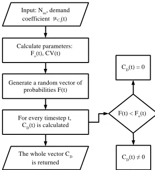
The flow chart of the stochastic algorithm implementation is shown in Figure 3. The main inputs of the algorithm are the mean demand coefficient pattern 𝜇𝐶_𝐷(𝑡)and the number of users NUs. 𝜇𝐶_𝐷(𝑡)

Figure 2: Flow chart of the implemented algorithm

For every time step a value of the probability F is generated in the interval (0,1). The generated probability is then confronted with the corresponding Fo(t). If F(t)<Fo(t) the result will be CD(t) = 0,

otherwise it will be calculated according to Eq.(12).

Then a vector containing a synthetic daily demand coefficient pattern is returned for the specific inputted pattern and the considered NUs.

3

A practical application

The proposed methodology allows to generate synthetic demand coefficient patterns in conditions of data scarcity. In these situations, some works in scientific literature can provide the basis to estimate some peculiar points of a daily demand coefficient pattern. By means of the piecewise interpolations method shown in the previous sections, it is possible to obtain a mathematical curve that mimics the average demand coefficient daily trend, congruently to the set fixed points.

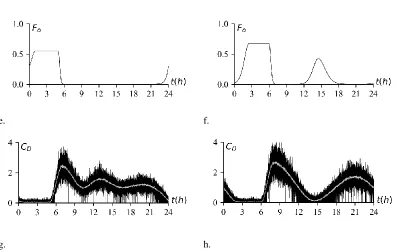
As an example, the results inherent to the demand pattern generation of two cases are herein reported in Figure 3. Detailed information about the cases parameters is shown in Table 1.

Case 1 Case 2

Peak number 3 2

Peak times 7:00, 13:00, 20:00 8:00, 21:00 Peak multiplier 1.00, 0.65, 0.50 1.00, 0.65

𝑁𝑢𝑠 1200 800

Minimum demand period 1:00÷5:00 2:30÷6:00 Table 1: Summary of the data of the two generated cases

In Figure 3, a.-b. it is possible to see that the algorithm is able to find plausible positions for the unknown valleys, providing congruent average daily demand coefficient trends (continuous line) by means of the PCHIP interpolators. Furthermore, the mean of the generated patterns (dotted line) over the 50 days by means of the Monte Carlo (MC) shows a good accordance to the interpolated one. The trend itself presents an unnatural and overly smooth shape due to its mathematical origin, but it preserves all the typical peculiarities discussed in Section Errore. Il segnalibro non è definito..

CD(t) ≠ 0 CD(t) = 0 Calculate parameters:

Fo(t), CV(t)

Generate a random vector of probabilities F(t) Input: Nus, demand coefficient (t)

For every timestep t, CD(t) is calculated

The whole vector CD is returned

F(t) < Fo(t)

According to the interpolated trend are then generated the probability of null demand with Eq.(9) and the CV with Eq.(11) along the day that are shown respectively in Figure 3, c.-d. and Figure 3, e.-f

Finally, the daily trends for 50 days are generated according to Eq.(12) and are shown in Figure 3, g. and h., overlapped by the time averaged demand coefficient pattern over the simulation period.

4

Conclusions

In this work has been proposed an approach to extrapolate daily demand patterns from some known points that can be estimated by several approaches in scientific literature. The proposed methodology uses Piecewise Cubic Hermite Interpolating Polynomials to fit a continuous curve to the known points and estimate the unknown ones by means of an optimization approach.

The resulting average demand coefficient pattern is then used to perform a stochastic demand generation using a Monte Carlo approach. The stochastic generation follows an approach based on a mixed distribution that contemplates two random variables: a discrete one that models the probability of null water demand, and a continuous one that models the demand when it is not zero.

The interpolated pattern and the related estimated variables, such as the Coefficient of Variation and the probability of null water demand have obviously a overly smooth shape due to their mathematical origin, but they preserve the typical desired characteristics of a real demand pattern, such as peaks and valleys. They anyhow provide additional flexibility allowing the decision maker to model the demand pattern in every aspect even in conditions of data scarcity.

The proposed method has been implemented in Python to facilitate the use of this kind of approaches inside water simulation workflows and to generate demand patterns directly into EPANET input files.

a. b.

e. f.

g. h.

Figure 3: Results of the demand generation for the two cases, respectively: a., b. – overlapping of the average generated patterns with the interpolated one; c., d. – coefficient of variation; e., f. – probability of null water demand; g., h. – generated patterns versus the average pattern

References

[1] S. Buchberger and L. Wu, “Model for Instantaneous Residential Water Demands,” J. Hydraul. Eng., vol. 121, no. 3, pp. 232–246, Mar. 1995.

[2] E. J. M. Blokker, J. H. G. Vreeburg, and J. C. Van Dijk, “Simulating residential water demand with a stochastic end-use model,” Journal of Water Resources Planning and Management, vol. 136, no. 1, pp. 19–26, 2009.

[3] R. Gargano, C. Tricarico, G. del Giudice, and F. Granata, “A stochastic model for daily residential water demand,” Water Science and Technology: Water Supply, vol. 16, no. 6, pp. 1753– 1767, Dec. 2016.

[4] L. A. Rossman, EPANET 2 USERS MANUAL. 2000.

[5] H. E. Babbitt, Sewerage and sewage treatment. John Wiley & Sons, Incorporated, 1922. [6] G. de Marinis, R. Gargano, and C. Tricarico, “Water Demand Models for a Small Number of Users,” 2006, pp. 1–14.

[7] R. Gargano, C. Tricarico, F. Granata, S. Santopietro, and G. de Marinis, “Probabilistic Models for the Peak Residential Water Demand,” Water, vol. 9, no. 6, p. 417, Jun. 2017.

[8] C. Tricarico, G. de Marinis, R. Gargano, and A. Leopardi, “Peak residential water demand,” Proceedings of the Institution of Civil Engineers - Water Management, vol. 160, no. 2, pp. 115–121, Giugno 2007.

[10] J. M. A. Alkasseh, M. N. Adlan, I. Abustan, H. A. Aziz, and A. B. M. Hanif, “Applying Minimum Night Flow to Estimate Water Loss Using Statistical Modeling: A Case Study in Kinta Valley, Malaysia,” Water Resources Management, vol. 27, no. 5, pp. 1439–1455, Mar. 2013.

[11] M. Farley and S. Trow, Losses in water distribution networks: a practitioner’s guide to assessment, monitoring and control. London: IWA Publ, 2003.

[12] S. G. Buchberger and G. Nadimpalli, “Leak Estimation in Water Distribution Systems by Statistical Analysis of Flow Readings,” Journal of Water Resources Planning and Management, vol. 130, no. 4, pp. 321–329, 2004.

[13] H. Akima, “A new method of interpolation and smooth curve fitting based on local procedures,” Journal of the ACM (JACM), vol. 17, no. 4, pp. 589–602, 1970.

[14] R. L. Dougherty, A. S. Edelman, and J. M. Hyman, “Nonnegativity-, monotonicity-, or convexity-preserving cubic and quintic Hermite interpolation,” Mathematics of Computation, vol. 52, no. 186, pp. 471–494, 1989.

[15] F. N. Fritsch and R. E. Carlson, “Monotone piecewise cubic interpolation,” SIAM Journal on Numerical Analysis, vol. 17, no. 2, pp. 238–246, 1980.

[16] D. F. Shanno and P. C. Kettler, “Optimal conditioning of quasi-Newton methods,” Mathematics of Computation, vol. 24, no. 111, pp. 657–664, 1970.

[17] C. G. Broyden, “The convergence of a class of double-rank minimization algorithms: 2. The new algorithm,” IMA Journal of Applied Mathematics, vol. 6, no. 3, pp. 222–231, 1970.