Optimal Linear Codes Over GF(7) and GF(11) with Dimension 3

(1)

Vol. 10, No. 1 (2015), pp 11-22 DOI: 10.7508/ijmsi.2015.01.002

Optimal Linear Codes Over

GF

(7)

and

GF

(11)

with

Dimension

3

M. Emami∗, L. Pedram

Department of Mathematics, University of Zanjan, Zanjan, I. R. Iran.

E-mail: [email protected] E-mail: [email protected]

Abstract. Letnq(k, d) denote the smallest value ofnfor which there

exists a linear [n, k, d]-code over the Galois fieldGF(q). An [n, k, d]-code whose length is equal to nq(k, d) is calledoptimal. In this paper we

present some matrix generators for the family of optimal [n,3, d] codes over GF(7) and GF(11). Most of our given codes in GF(7) are non-isomorphic with the codes presented before. Our given codes inGF(11) are all new.

Keywords: Linear codes, Optimal codes, Griesmer bound.

2010 Mathematics Subject Classification: 68P30, 94A29.

1. _Introduction

Let Vn(q) be the vector space of all ordered n-tuples over GF(q) (Galois

field of q elements). Each subspace of Vn(q) is called a linear code. By an

[n, k, d]-code of lengthnand dimensionkoverGF(q) we mean ak-dimensional subspace of Vn(q) with minimum Hamming distance d. Sometimes we use

the term [n, k]-code if the minimum distance d is not under consideration. Optimizing any one of the parametersn, k and d, when the other two values are given is one of the main problems in coding theory. These problems over a

∗_{Corresponding Author}

Received 31 January 2013; Accepted 13 September 2014 c

2015 Academic Center for Education, Culture and Research TMU

11

(2)

fixedGF(q) can be characterized as follows [7,9,11]:

1. What is the maximum value ofd(denoted bydq(n, k)) for which there exists

an [n, k, d]-code?

2. What is the minimum value ofn(denoted bynq(k, d)) for which there exists

an [n, k, d]-code?

3. What is the maximum value ofk(denoted bykq(n, d)) for which there exists

an [n, k, d]-code?

For a literature backlog of this topic whenq= 2,3,5 and 7 one is refereed to [2,3,4,5,7,9,14,15,17,18,21,22,23]. In this paper we consider the problem for the case of codes overGF(7) andGF(11). In section 2 we give a brief review of our method. In Section 3 we give some basic necessary preliminaries. In Section 4 and 5 we study the value of functions n7(k, d) andn11(k, d) for k ≤3 and some values ofd.

2. _{A Brief Review of Our Method}

In all parts of this study we followed a random process to obtain generator matrices for specified codes. For a givenk andd, the length nof the optimal code can be obtained from the Griesmer bound and the existence of a possible [n, k, d]-code can be investigated by the MacWilliams identities. In case of nonexistence, we try to produce an [n+ 1, k, d]-code. In case of existence, the weight distributions given by MacWilliams identities help us to produce the code. We generate matrices of size k×n by a random process (based on a computer programming), we then test each of these matrices to be a generator matrix for a specific [n, k, d]-code. Since the parameters are small, in case of necessity we may produce all code words to find the weight distributions of the code to see whether the weight distributions satisfy the MacWilliams identities. In quasi-cyclic codes we studied only the cases where n is a multiple of k. Now sincen=ks, for some positive integer “s”, we produced the first row of each of thescirculant matricesGi of sizek×k, by the same random process,

whereG= [G1|G2| · · · |Gs] by the notations given in the corresponding section,

is the generating matrix of a code. The remaining rows of each Gi would fill

cyclically. In last step the weight distributions should be tested.

As an example theQC[32,4,25]-code is consist of 8 circulant matrices of size 4×4, which is built as above. Gulliver method, as cited in Grassl code table [6], gives a different construction for this code which is based on two polynomials of degree 15 to produce the first rows of two matrices of sizes 4×16.

Also, it is important to note that in [4] as cited in Grassl table [6], the study uses the following method: given the parameters n and k, the optimality of code is focused ond(minimum distance), whereas in our papers, we employ a

(3)

different method: given the parameterskandd, the optimality is focused onn. Sure both methods reach to a unique optimal code, while the methods are com-pletely different. In quasi cyclic codes we tried to find the generating matrices, where their weight distributions satisfy MacWilliams identities, meanwhile the other references such as [4] have a different approach.

For more emphasis on the originality of our methods and our results we tested some of our generator matrices, for any possible isomorphism, compared with the generator matrices given in Grassl table [6]. So we computed the weight distributions of some of the codes given in Grassl tables by a computer programming and found that they are all completely different.

For example our QC[20,4,15] and [32,4,25]-codes are both non-isomorphic with the sameQC[20,4,15] and [32,4,25] codes given in Grassl table, as their weight distributions are different. One of the [28,4,21]-codes and two of the [24,4,18]-codes given in Grassl table, are all non-isomorphic from our corre-sponding codes (their weight distributions are different).

3. _{Preliminaries}

let w(x) denotes the Hamming weight of a vector x. That is the number of nonzero entries inx. For a linear code, the minimum distancedis equal to the smallest value ofw(x) whenxrange over all nonzero codewords. LetC be an [n, k]-code and letAi andBibe the number of codewords of weightiinCand

in dual codeC⊥, respectively [9]. Now note that:

Theorem 3.1. (The MacWilliams identities[19]). LetCbe an[n, k]-code over GF(q). Then the Ai,s andBi,s satisfy

n−t X

j=0 _n₋_j

t

Aj =qk−t t X

j=0 _n₋_j

n−t

Bj. (3.1)

fort= 0,1, . . . , n.

Lemma 3.2. [9]. For an[n, k, d]-code overGF(q),Bi = 0for each value of i

(where1≤i≤k) such that there does not exist an [n−i, k−i+ 1, d]-code.

Lemma 3.3. [10] : Let C be an [n, k, d]-code over GF(q) with k ≥2 , and

with weight enumeratorPn

i=0Aizi . Then

(i) if xand y are a linearly independent pair of codeword ofC ,

w(x) +w(y)≤qn−qd+d, (3.2) (ii) Ai= 0 fori > q(n−d).

Corollary 3.4. (I) LetC be an[n, k, d]-code overGF(7) withk≥2. Then : (i) ifxandyare a linearly independent pair of codewords ofC, thenw(x) + w(y)≤7n−6d,

(ii) Ai= 0 fori >7(n−d),

(4)

(iii)Ai = 0or6 fori >1/2(7n−6d),

(iv) ifAi>0, thenAj = 0forj >7n−6d−i andi6=j;

(II)If C be an [n, k, d]-code overGF(11)with k≥2, then :

(i) ifxandyare a linearly independent pair of codewords ofC, thenw(x) + w(y)≤11n−10d,

(ii) Ai= 0 fori >11(n−d),

(iii)Ai = 0or10 fori >1/2(11n−10d),

(iv) ifAi>0, thenAj = 0forj >11n−10d−i andi6=j.

Proof. (I) (i) and (ii) are immediate from Lemma 2.

(iii) Suppose i > 1/2(7n−6d). By part (i), there cannot be two linearly independent codeword of weighti. So there are either no codeword of weight ior just six (x, 2x, 3x, 4x, 5xand 6xfor somex∈C).

(iv) By part (i), there cannot exist codeword of weight i and j, with i 6= j, satisfyingi+j >7n−6d.

(II) The same way of (I).

Definition 3.5. Let C be an [n, k, d]-code overGF(q). If we delete a given coordinate from all codewords of Cthen we have a punctured codeofC. This code is an [n−1, k, d−1]-code. The set of all codewords ofC having zero in a given coordinate position and then deleting that coordinate is a code called a shortened codeofC. This code is an [n−1, k−1, d]-code, provided not the given position in all code wordsCis zero [9].

Lemma 3.6. [9](i)nq(k, d)≤nq(k, d+ 1)−1,

(ii) nq(k, d)≥nq(k, d−1) + 1,

(iii)nq(k, d)≤nq(k+ 1, d)−1,

(iv)nq(k, d)≥nq(k−1, d) + 1.

Definition 3.7. LetGbe the generator matrix of a linear [n, k, d]-codeCover GF(q). Then theresidual codeofC with respect to a codewordc, denoted be Res(C, c), is the code generated by the restriction ofGto the columns wherec has a zero entry [9].

Lemma 3.8. [9]SupposeC is an[n, k, d]-code overGF(q)and supposec∈C has weightw, whered > w(q−1)/q. Then Res(C, c)is an[n−w, k−1, d0_]-code withd0_≥_d₋_w₊_d_w/q_e_.

(dxedenotes the smallest integer greater than or equal to x.)

Corollary 3.9. Suppose C is an [n, k, d]-code over GF(q), and let c be a

codeword of weightd. Then Res(C, c)is an[n−d, k−1,dd/qe]-code [9].

Theorem 3.10. (The Griesmer bound ). Let gq(k, d)denote the sum

expres-sionPk−1 i=0dd/q

i_e_{. Then} _n

q(k, d)≥gq(k, d).

The class of codes which satisfy the Griesmer bound is addressed ascodes of type BV. Such codes can be produced by certain puncturings of concatenations

(5)

of simplex codes and one can show that, for givenqandk, the Griesmer bound is attained for all sufficiently larged. The following theorem gives a necessary and sufficient condition for the existence of a code of typeBV [7,11,16].

Theorem 3.11. For given q, k andd, write d =sqk−1₋Pp

i=1qui−1, where s=dd/qk−1e,k > u1≥u2≥. . .≥up≥1, and at mostq−1 of u,is take any

given value. Then there exists a [gq(k, d), k, d]-code of type BV if and only if Pmin(s+1,p)

i=1 ui≤sk.

4. _{Optimal Codes with} q= 7,11 _{of Dimension}≤3

Fork≤2, it follows from Theorem 11 thatn7(k, d) =g7(k, d) for alld. Thus n7(1, d) =dandn7(2, d) =d+dd/7efor alld.

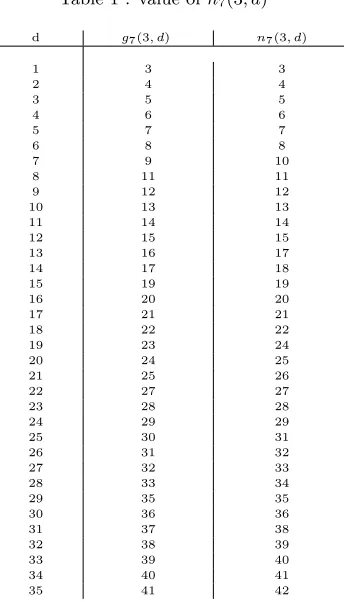
Fork= 3, Theorem 11 implies thatn7(3, d) =g7(3, d) ford≥36. The remaining values ofdare listed in Table 1.

Table 1 : value ofn7(3, d)

d g7(3, d) n7(3, d)

1 3 3

2 4 4

3 5 5

4 6 6

5 7 7

6 8 8

7 9 10

8 11 11

9 12 12

10 13 13

11 14 14

12 15 15

13 16 17

14 17 18

15 19 19

16 20 20

17 21 21

18 22 22

19 23 24

20 24 25

21 25 26

22 27 27

23 28 28

24 29 29

25 30 31

26 31 32

27 32 33

28 33 34

29 35 35

30 36 36

31 37 38

32 38 39

33 39 40

34 40 41

35 41 42

Theorem 4.1. (i)n7(3,5)≤7, (ii)n7(3,6)≤8, (iii) n7(3,11)≤14.

(6)

Proof. (i) The matrix 

 

0 4 3 2 0 3 1 6 0 0 3 2 1 3 5 2 4 2 1 5 1



 

generates [7,3,5]-code overGF(7).

(ii) it is shown in [11] that [q+ 1,3, q−1]-code exists overGF(q). In particular, there exists [8,3,6]-code overGF(7). Its generator matrix is



 

4 4 3 2 1 0 3 0 4 0 1 5 4 3 6 0 5 6 3 5 0 0 5 1



 

(iii) The matrix



 

1 3 2 1 1 1 2 3 0 1 3 1 3 3 5 0 4 1 5 2 5 5 0 1 2 6 2 5 2 1 2 6 3 4 6 4 4 1 1 6 2 3



 

generates [14,3,11]-code overGF(7) and its weight distribution isA11= 162,A12=

60,A13= 66 andA14= 54.

Theorem 4.2. n7(3,10)≤13.

Proof. The matrix 

 

0 6 1 6 2 5 1 0 1 5 0 6 2 2 4 6 3 1 6 1 6 1 2 2 1 4 2 1 4 3 2 4 2 1 3 2 0 6 3



 

90,A12= 66 andA13= 60.

Theorem 4.3. (i)n7(3,7)>9, (ii)n7(3,35)>41.

Proof. (i) Ifqis odd, an [q+k−1, k]-code MDS does not exist [1]. Then [9,3,7]-code does not exist. This matrix generates [10,3,7]-code with weight distributionA7= 54, A8= 108,A9= 102 andA10= 78



 

3 1 1 3 1 2 0 1 1 4 2 6 3 6 5 0 1 6 5 6 1 4 1 6 6 0 0 1 0 6



 

(ii) Ford= (k−2)qk−1₋₍_k₋₁₎_qk−2_,_n

q(k, d)> gq(k, d) holds forq≥k,k= 3,4,5 [12]. Then we have fork= 3 andq= 7, [41,3,35]-code dose not exist.

Theorem 4.4. n7(3,13)>16.

Proof. Suppose, for a contradiction, that there exist a [16,3,13]-codeC overGF(7). Since there do not exist codes overGF(7) with parameters [15,3,13] and [14,2,13], it follows from Lemma 2 that B1 =B2 = 0. The first three MacWilliams identities (Theorem 1) become,

A13+A14+A15+A16= 342, A14+ 2A15+ 3A16= 258,

(7)

A15+ 3A16= 210.

By Lemma 8, the residual code ofCwith respect to a codeword of weight 15 would be a [1,2,1]-code, which dose not exist. soA15= 0. Bearing in mind that eachAi must be a nonnegative integer multiple of 6 (because ifxis a nonzero codeword, then so also are 2x,3x,4x,5xand 6xof the same weight). The last equation givesA16= 70 that is not divisible by 6.

This matrix generates [17,3,13]-code



 

4 6 0 4 5 5 5 5 1 6 6 6 4 1 0 6 5 2 6 4 5 0 2 5 6 0 5 5 1 2 1 2 3 3 6 1 5 3 3 6 1 2 6 3 2 5 2 5 4 5 3



 

and its weight distribution isA13 = 60,A14 = 126,A15 = 78,A16= 42 andA17=

36.

Theorem 4.5. n7(3,21)>25.

Proof. Suppose there exist an [25,3,21]-codeCoverGF(7).By Lemma 2,B1=B2= 0. The MacWilliams identities become,

(a)A21+A22+A23+A24+A25= 342, (b)A22+ 2A23+ 3A24+ 4A25= 168, (c)A23+ 3A24+ 6A25= 252.

By Lemma 8,A22=A23=A24= 0. By Corollary 4(iii),A25= 0 or 6, this contradicts (c).

This matrix generates [26,3,21]-code and its weight distribution isA21= 108,A22= 108,A23= 60,A24= 42,A25= 12 andA26= 12.

0 1 2 3 6 3 2 6 3 5 4 5 4 5 5 1 5 2 4 3 0 0 2 3 0 4 4 2 2 4 1 2 5 4 6 5 0 2 5 4 0 3 2 4 1 1 6 6 4 3 3 4 4 5 1 4 3 5 0 6 2 2 1 1 6 0 0 0 3 5 4 3 1 0 1 3 1 1

Theorem 4.6. n7(3,28)>33.

Proof. Suppose there exist an [33,3,28]-codeCoverGF(7).By Lemma 2,B1=B2= 0. The MacWilliams identities become,

(a)A28+A29+A30+A31+A32+A33= 342, (b)A29+ 2A30+ 3A31+ 4A32+ 5A33= 126, (c)A30+ 3A31+ 6A32+ 10A33= 252,

By Lemma 8,A29=A30=A31=A32= 0. By Corollary 4(iii),A33= 0 or 6, which

contradicts (c).

Theorem 4.7. (i)n11(3,5)≤7, (ii)n11(3,7)≤9, (iii) n11(3,13)≤16,

(iv)n11(3,14)≤17.

Proof. (i) This matrix generates [7,3,5]-code and its weight distribution isA5= 210, A6= 420 andA7= 700.



 

3 9 10 0 9 3 4 6 9 5 3 8 10 9 7 1 6 4 8 9 4



 

(8)

(ii) This matrix generates [9,3,7]-code and its weight distribution isA7= 360,A8= 360 andA9= 610. Another generator matrix is given in section 4.



 

10 4 5 1 1 1 1 3 8 1 9 7 1 1 0 8 0 7 2 1 10 2 4 6 9 9 0



 

(iii) The matrix



 

0 2 1 10 9 1 10 6 4 5 2 3 0 5 10 4 1 4 10 1 7 2 4 6 0 3 2 3 5 2 6 6 4 7 5 3 9 5 9 2 10 1 6 0 7 6 4 9



 

generates [16,3,13]-code overGF(11) and its weight distribution isA13= 300,A14= 300,A15= 420 andA16= 310.

(iv) The matrix



 

3 6 0 1 8 10 8 3 3 2 5 4 4 5 6 3 3 6 6 7 8 4 5 2 8 0 8 10 10 1 9 2 7 9 3 4 9 1 8 1 3 2 5 8 7 1 0 10 7 6 6



 

340,A16= 340 andA17= 310.

5. _{Quasi-Cyclic Codes}

QC codes are a generalization of cyclic codes whereby a cyclic shift of a codeword byppositions results in another codewords. It can be shown thatpmust be divisor ofn[8]. Therefore, cyclic codes are QC codes withp= 1. With a suitable

permutation of coordinate, many QC codes can be characterized in terms ofm×m

circulant matrices, so the blocklength,n, is a multiple ofm,n=mp. The generator matrix can then be represented asG= [C0, C1, C2, . . . , Cp−1]. Ciis an m×m circulant matrix of the form

C=        

c0 c1 c2 . . . cm−1 cm−1 c0 c1 . . . cm−2 cm−2 cm−1 c0 . . . cm−3

. .

. ... ... ...

c1 c2 c3 . . . c0

       

where each successive row is a right cyclic shift of the previous one. These codes are a subclass of the more general 1-generator QC codes [20], which is in turn a subclass of all QC codes.

This has been confined mainly to the casem=k. Ans-QC [sk, k]-codes has a generator matrix of the formG= [G1|G2|. . .|Gs], where eachGiis ak×k circulant matrix. The matrixG1 is usually taken to be the identity matrixI [8]. In this section we produce generator matrix of QC [sk, k]-codes withk= 3 overGF(7) andGF(11).

Theorem 5.1. (i)n7(3,4) = 6, (ii)n7(3,9) = 12, (iii)n7(3,12) = 15, (iv)n7(3,14) = 18.

(9)

Proof. There exist codes with parameters [6,3,4], [12,3,9], [15,3,12] and [18,3, 14]-codes. The weight distributions and generators matrices are :

[6,3,4] A0= 1,A4= 90,A5= 108 andA6= 144; (422|533);

[12,3,9] A0= 1,A9= 102,A10= 90,A11= 90 andA12= 60; (322|633|022|046);

[12,3,9] A0= 1,A9= 96,A10= 108,A11= 72 andA12= 66; (532|066|212|040);

[15,3,12] A0= 1,A12= 180,A13= 90,A14= 0 andA15= 72; (205|021|642|054|346);

[18,3,14]-A0= 1,A14= 90,A15= 90,A16= 108,A17= 18 andA18= 36; (322|633|022|046|450|244);

[18,3,14]-A0= 1,A14= 90,A15= 108,A16= 54,A17= 72 andA18= 18;

(515|212|343|531|630|500).

Theorem 5.2. (i)n7(3,17) = 21, (ii)n7(3,19) = 24, (iii)n7(3,22) = 27 and (iv) n7(3,27) = 33.

Proof. There exist codes with parameters [21,3,17], [24,3,19], [27,3,22] and [33,3,27] codes. The weight distributions and generators matrices are :

[21,3,17]-A0= 1,A17= 126,A18= 168,A19= 0,A20= 0 andA21= 48; (002|521|321|640|434|633|624);

[24,3,19]-A0= 1,A19= 72,A20= 108,A21= 90,A22= 18,A23= 54 andA24= 0; (255|520|452|045|423|544|546|202);

[24,3,19]-A0= 1,A19= 108,A20= 36,A21= 84,A22= 108,A23= 0 andA24= 6; (164|566|346|114|110|311|552|034);

[27,3,22]-A0= 1,A22= 126,A23= 90,A24= 102,A25= 0,A26= 0 andA27= 24; (646|623|565|101|354|136|605|130|043);

[33,3,27]-A0 = 1, A27 = 96, A28 = 126, A29 = 54, A30 = 42, A31 = 18, A32 = 0 andA33= 6;

(245|664|023|432|513|404|056|104|543|051|246);

[33,3,27]-A0 = 1, A27 = 54, A28 = 216, A29 = 18, A30 = 24, A31 = 18, A32 = 0 andA33= 12;

(426|210|060|533|461|105|453|552|242|305|022).

Theorem 5.3. (i)n7(3,30) = 36, (ii)n7(3,32) = 39and (iii)n7(3,35) = 42.

Proof. There exist codes with parameters [36,3,30], [39,3,32] and [42,3,35] codes. The weight distributions and generators matrices are :

[36,3,30]-A0= 1,A30= 168,A31= 90,A32= 54,A33= 6,A34= 18,A35= 0 and A36= 6;

(515|146|605|153|130|200|012|253|302|251|411|434);

(10)

[36,3,30]- A0 = 1,A30= 168,A31= 72,A32= 90,A33= 0,A34= 0,A35= 0 and A36= 12;

(503|166|402|265|351|022|352|565|510|535|312|631);

[39,3,32]-A0 = 1,A32= 90,A33= 108,A34= 90,A35 = 18,A36= 12,A37= 18, A38= 0 andA39= 6;

(601|164|426|210|060|533|461|105|453|552|242|305|022);

[39,3,32]-A0 = 1,A32= 90, A33= 114, A34 = 72,A35= 36, A36 = 6,A37= 18, A38= 0 andA39= 6;

(414|660|442|120|406|553|030|543|056|106|541|561|661);

[42,3,35]-A0 = 1,A35= 162, A36= 78, A37 = 54,A38= 18, A39 = 24,A40 = 0, A41= 0 andA42= 6;

(400|423|320|224|463|606|145|221|312|334|020|155|402|612);

[42,3,35]- A0 = 1, A35 = 162, A36 = 84,A37= 126, A38 = 0,A39 = 0,A40 = 0, A41= 0 andA42= 6;

(350|120|212|051|256|144|463|066|564|545|432|340|233|005).

Generator matrices of twoQC-codes that meet the Griesmer bound are given in the following,

[45,3,38]-A0= 1,A38= 180,A39= 120,A40= 36,A41= 0,A42= 0,A43= 0, A44= 0,A45= 6.

(500|524|042|043|545|252|513|206|636|153|163|036|440|121|454).

[48,3,41]-A41= 288,A42= 48,A43= 0,A44= 0,A45= 0,A46= 0,A47= 0, A48= 6

(643|406|332|216|533|525|003|263|521|660|103|240|415|014|136| 121).

[6,3,4]-A0= 1,A4= 150,A5= 420 andA6= 760; (5 2 7|10 3 4);

[9,3,7]-A0= 1,A7= 360,A8= 360 andA9= 610; (9 1 8|4 1 3|5 6 5);

[12,3,10]-A0= 1,A10= 660,A11= 120 andA12= 550; (3 6 10|6 6 9|4 6 8|5 5 10).

[15,3,12]-A0= 1,A12= 210,A13= 420,A14= 330 andA15= 370; (7 10 4|6 4 10|0 10 4|2 6 5|6 7 6);

(11)

[18,3,15]-A0= 1,A15= 400,A16= 330,A17= 300 andA18= 300; (0 4 8|0 3 3|3 9 9|1 8 2|8 2 5|1 6 1);

[21,3,18]-A0= 1,A18= 630,A19= 210,A20= 210 andA21= 280; (6 2 1|1 1 2|1 5 4|8 10 10|6 4 9|7 1 10|2 2 9).

[27,3,23]-A0= 1,A23= 390,A24= 280,A25= 330,A26= 180 andA27= 150; (10 5 1 |0 5 3 | 2 1 7 | 0 10 4 | 2 0 9 | 2 7 9 | 2 5 7 | 2 6 1 |

9 10 6);

[30,3,26]-A0= 1,A26= 540,A27= 300,A28= 210,A29= andA30= 120; (9 4 4 | 2 4 9 | 10 0 8 | 3 3 0 | 8 4 3 | 0 9 6 | 7 6 4 | 2 3 7 | 10 2 3|8 6 1);

[39,3,34]- A0 = 1, A34 = 450, A35 = 360,A36 = 220, A37 = 90, A38 = 150 and A39= 60;

(5 3 6 | 4 4 0 | 2 9 3 | 2 6 1 | 4 5 3 | 1 1 4 | 5 9 2 | 9 7 9 | 6 10 8|3 7 10|7 1 3|3 5 7|3 8 6).

Acknowledgments

The authors would like to give their best thanks to the anonymous referee for his/her valuable comments to promote this work.

References

1. T. L. Alderson, Extending MDS codes,Annals of combinatorics,9, (2005), 125-135. 2. M. Amini, Quantum error-correcting codes on Abelian groups,Iranian journal of

math-ematical sciences and informations,5(1), (2010), 55-67.

3. I. Boukliev, S. Kapralov, T. Maruta, M. Fukui, Optimal linear codes of dimension 4 over F5,IEEE Transactions on Information Theory,43, (1997), 308-313.

4. R. N. Daskalov, T. A. Gulliver, Bounds in Minimum Distance for Linear Codes over GF(7),JCMCC,36, (2001), 175-191.

5. A. Cheraghi, On the pixel expansion of hypergraph acess structures in visual cryptogra-phy schemes,Iranian journal of mathematical sciences and informations,5(2), (2010), 45-54.

6. M. Grassl, Tables of minimum-distance bounds for linear codes, http://www.codetable.de/.

7. P. P. Greenough, R. Hill, Optimal linear codes overGF(4),Discrete Mathematics,125, (1994), 187-199.

8. P. P. Greenough, R. Hill, Optimal ternary quasi-cyclic codes,Designs, Codes and Cryp-tography,2, (1992), 81-91.

9. R. Hill, D. E. Newton, Optimal ternary linear codes,Codes and Cryptography,22, (1992), 137-157.

10. R. Hill, D. E. Newton, Some optimal ternary linear codes,Ars Combinatoria,25, (1988), 61-72.

(12)

11. R. Hill,Optimal linear codes, in: C. Mitchell. ed., Pro. 2nd IMA Conf. on Cryptography and Coding (Oxford Univ. Press, Oxford, (1992)) 75-104.

12. R. Hill, E. Kolev, A survey of recent results on optimal linear codes, Combinatorial Designs and their Application, CRC Research Notes in Mathematics,403, (1999), 127-152.

13. A. Klein, On codes meeting the Griesmer bound, Discrete Mathematics,274, (2004), 289-297.

14. I. Landjev, Optimal linear codes of dimension 4 overF5,Lecture Notes in Comp. Science,

1225, (1997), 212-220.

15. I. Landjev, A. Rousseva, T. Maruta and R. Hill, On optimal codes over the field with five elements,Codes and Cryptography,29, (2003), 165-175.

16. F. J. MacWilliams, N. J. A. Sloan, The theory of error correcting codes, Amsterdam. North Holland.

17. T. Maruta, On the minimum length of q-ray linear codes of dimension four, Discrete Mathematics,208/209, (1999), 427-435.

18. T. Maruta, I. N. Landjev, A. Rousseva, On the minimum size of some minihypers and related linear codes,Designs, Codes and Cryptography,34, (2005), 5-15.

19. V. Pless,Introduction to the theory of error-correcting codes, New York; Wiley (1982). 20. G. E. S´eguin, G. Drolet,The theory of 1-generator quasi-cyclic codes, Royal Military

College of Canada, Kingston, ON, (1991).

21. H. C. A. VanTilborg, The smallest length of binary 7-dimensional linear codes with precribed minimum distance,Discrete Mathematics,33, (1981), 197-207.

22. T. Verhoef, An updated table of minimum distance bounds for binary linear codes,IEEE Transactions on Information Theory,33, (1987), 665-680.

23. H. N. Ward, The nonexistence of a [207,4,165]-code over GF(5), Designs, Codes and Cryptography,22, (2001), 139-148.