Volume 8, 2018, Pages 70–83
TNC’18. Trusted Numerical Computations
Enhancing monotonicity checking in parametric
interval linear systems
Iwona Skalna
1and Milan Hlad´ık
21
AGH University of Science and Technology, Department of Applied Computer Science,
Krak´ow, Poland [email protected]
2
Charles University, Faculty of Mathematics and Physics, Department of Applied Mathematics,
Malostransk´e n´am. 25, 11800, Prague, Czech Republic [email protected]
Abstract
Solving systems of parametric linear equations with parameters varying within closed intervals is a hard computational problem. However, we may reduce the problem dimension and thus make the problem more tractable by utilizing the monotonicity of the solution components with respect to the parameters. In this paper, we propose two improvements of the standard monotonicity checking techniques. The first improvement relies on creating a system with original variables and their derivatives as unknowns, and the second one employs the so-called p-solution. By a series of numerical experiments we show that the improved monotonicity approach outperforms the standard one.
1
Introduction
In solving real-life problems, we often deal with data that are not know exactly due to various kinds of inexactness – measurement errors, incomplete knowledge, data estimation etc. In this paper, we assume that lower and upper bounds on uncertain data are known; i.e., we assume that we are dealing with interval valued quantities. Using intervals is advantageous because of their ability to track rounding and truncation errors and what follows to produce guaranteed solutions. However, due to the so-called dependency problem, classical interval computations often lead to large overestimation which makes their results irrelevant. Therefore, we address here a more general problem with dependencies between interval entries. More specifically, we focus on solving systems of linear equations with entries dependent on parameters varying within prescribed intervals.
Formally, consider ann-dimensional system of linear equations
A(p)x=b(p),
pk ∈pk = [pk, pk]. Thus, instead of a single parametric linear system, we have the following family of parametric linear systems
A(p)x=b(p), p∈p, (1)
wherep= (p1, . . . , pK) andp= (p1, . . . ,pK)T.
As a special case, we will also discuss systems with affine-linear dependencies, meaning that the entries ofA(p) and b(p) are affine-linear functions of parameters. In this case, A(p) and b(p) can be expressed as
A(p) = K X
k=1
A(k)p
k, b(p) = K X
k=1
b(k)p
k,
whereA(k)∈Rn×n
andb(k)∈Rn are fixed and known a priori.
The solution set of the system (1) is usually defined as the set of solutions to all systems from the family (1), i.e.,
Σ,{x∈Rn| ∃p∈p:A(p)x=b(p)}.
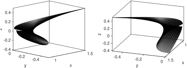
The (also called united) solution set Σ is hard to characterize, even for particular classes of the affine-linear case. For example, the explicit description of the symmetric systems (where the symmetry of the constraint matrix defines the linear dependencies) was developed, e.g., in [4, 18,19]. The general case of affine-linear dependencies was characterized by Popova [26] in particular. In such case, the shape of the solution set is described by quadrics (see Fig. 1). Handling Σ is computationally hard. Many questions, such as nonemptiness, boundedness or approximation, are NP-hard even for very special subclasses of problems; see [15,16,20].
Example 1. Consider the following three-dimensional parametric interval linear system with nonlinear dependencies in the right-hand side vector:
1 p1 p2
p1 2 p1
p2 p1 3
x=
1 p2
1
p2 1
, (2)
where p1 ∈ [0,1], p2 ∈[0,0.9]. The solution set of the system is depicted in Fig. 1. To give
a better idea, we display the solution set from two different perspectives there.
Let us now introduce some interval notation. An interval vector is defined as
x,{x∈Rn|x
i6xi 6xi, i= 1, . . . , n},
wherex, x∈Rn,x6x, are given. The midpoint of an intervalxis denoted byxc ,1
2(x+x),
and its radius byx∆, 1
2(x−x). The set ofn-dimensional interval vectors and the set ofn×m
interval matrices are denoted byIRn and IRn×m
, respectively. The smallest (w.r.t. inclusion) interval vector containing a bounded Σ is called aninterval hull of Σ and is denoted by✷Σ.
1.5
x 1 -0.4 y -0.2 0 -0.4 -0.2 0 0.2 0.4
z
1
x 1.5 0 -0.2
y -0.4 -0.4 -0.2 0 0.4
0.2
z
Figure 1: Solution set of system (2) viewed from different perspectives.
1.1
Monotonicity approach
A monotonicity approach was investigated by Kolev [7], Popova [22], Rohn [29], Skalna [34], and Skalna & Duda [38]. The idea is as follows. IfA(p) is non-singular, then the solution of the system A(p)x = b(p) is x = A(p)−1b(p). So, the solution is a real valued function of p,
i.e.,x=x(p). Ifxi(p) is monotonic onpwith respect to all parameters, then the smallest and largest values ofxi(p) onp (i.e., minimum and maximum of Σ inith coordinate) are attained at the respective endpoints ofp.
Ifxi(p) is monotonic with respect to some parameters only, then we can fix these parameters at the respective endpoints and then bound the range ofxi(p) on a box of a lower dimension. Suppose that
• xi(p) is nondecreasing onpin variablespk,k∈K1,
• xi(p) is nonincreasing onpin variablespk,k∈K2,
• xi(p) is non-monotonic onpin variablespk,k∈K3.
Define the restricted set of parametersp1 andp2 as follows
p1k =
pk k∈K1,
pk k∈K2,
pk k∈K3,
p2k =
pk k∈K1,
p
k k∈K2,
pk k∈K3,
Then
(✷Σ)
i = min{xi|x∈Σ}= min{xi| ∃p∈p
1:A(p)x=b(p)},
(✷Σ)i= max{xi|x∈Σ}= max{xi | ∃p∈p2:A(p)x=b(p)}. In this way, the computation reduces to two problems of smaller dimension.
The question now is how to check for monotonicity ofxi(p) in parameterpk. The standard way is to determine the sign of the partial derivative ∂xi(p)
∂pk onp. We can determine the sign of
∂xi(p)
∂pk for alli= 1, . . . , nby solving the following parametric interval linear system
A(p)∂x(p) ∂pk
=∂b(p) ∂pk
−∂A(p) ∂pk
In particular, for the affine-linear case, the system (3) takes the form
A(p)∂x(p) ∂pk
=b(k)−A(k)x(p), p∈p.
Since the vectorx(p) in (3) is not knowna priori, it is usually estimated by an outer interval enclosure of the solution set. That is, let x⊇Σ, and consider the parametric interval linear system
A(p)∂x(p) ∂pk
= ∂b(p) ∂pk
−∂A(p) ∂pk
x, x∈x, p∈p. (4)
For the affine-linear case, the system (4) takes the form
A(p)∂x(p) ∂pk
=b(k)−A(k)x, x∈x, p∈p. (5)
Letdbe an enclosure of the solution set of the system (4). Ifdi>0, thenxi(p) is nondecreasing inpk, and similarly ifdi60, thenxi(p) is nonincreasing inpk.
By solving the system (4) for eachk= 1, . . . , K, we obtain the interval vectorsd1, . . . ,dK. Provided that 06∈dki for everyk= 1, . . . , K andi= 1, . . . , n, we can compute the exact range of the solution set Σ as follows. For everyk= 1, . . . , K andi= 1, . . . , ndefine
p1k,i= (
p k d
k i >0, pk d
k i 60,
p2k,i= (
pk dki >0, pk dki 60.
By solving a pair of real linear systems of equations
A p1,i
x1=b p1,i
, (6a)
A p2,i
x2=b p2,i
, (6b)
we obtain
(✷Σ) i=x
1
i,
(✷Σ)i=x2i.
By solving n pairs of real linear systems (6), we obtain the range of the solution set in all coordinates, that is,✷Σ. The number of equations to be solved can be decreased by removing redundant vectors from the list
L=
p1,1, . . . , p1,n, p2,1, . . . , p2,n .
If only some of the partial derivatives have constant sign onp, then, in the worst case, instead of 2nreal systems, we must solve 2nparametric interval linear systems with a smaller number of interval parameters.
2
New approach
2.1
Augmented system
The first idea is to consider ∂x(p)/∂pk, k = 1, . . . , K, as additional variables in (3). This approach was suggested by prof. L. Kolev, however, as far as we know, the result was not published anywhere. For eachk= 1, . . . , K, we create the following parametric interval linear system
A(p) 0 ∂A(p)
∂pk A(p)
! x ∂x ∂pk
!
= ∂bb(p)(p) ∂pk
!
, p∈p, (7)
and solve it in order to obtain, hopefully narrower, bounds for ∂x
∂pk(p) overp. Then we proceed analogously as described in the previous section. Let us notice that for the affine-linear case, the system (8) takes the form
A(p) 0
A(k) A(p)
! x ∂x ∂pk
!
= b(p) b(k)
!
, p∈p, (8)
which is also a parametric interval linear system with affine-linear dependencies.
The presented modified version of the monotonicity approach eliminates the problem of the “lost of information”, however, instead we have to solve several systems which are twice larger than the original system. Since the basic version of the method is already quite expensive, hence for larger problems the modified method might be inefficient.
2.2
p
-solution
Below, we present a new approach to the “lost of information” problem, which relies on replacing x(p) in the right hand side of (3) with a more precise object. For this purpose, we employ the p-solution that was introduced by Kolev [13,14], and later studied by the authors in [39]. This type of solution has the parametric formx(p) =Lp+a, whereLis a realn×K-matrix andais an interval column vector. Substitutingx(p) with this type of solution, we obtain the following parametric interval linear system
A(p)∂x ∂pk
=b(p)−∂A(p) ∂pk
Lp−∂A(p) ∂pk
a, a∈a, p∈p, (9)
where the elements of interval vector a are treated as new interval parameters, independent fromp. In the affine-linear case, the linear system (9) takes the form
A(p)∂x ∂pk
=b(k)−A(k)Lp−A(k)a, a∈a, p∈p. (10)
2.3
Properties of
p
-solution approach
In this subsection, we consider the affine-linear case only. From many perspectives the system (10) is not more complicated than the original system (1).
Proposition 1. Consider the class of problems where matrices A(p), for all p ∈ p, are nonsingular and the solution set is convex resp. polyhedral for any right-hand side vectorb(p). Then the solution set of (10)is convex resp. polyhedral, too.
is convex resp. polyhedral. The image of A(k)a over a ∈ a is a zonotope, which is a convex
polyhedron. Due to linearity of the solutionx=A(p)−1b(p) with respect tob(p), we have that
the solution set of (10) is a Minkowski sum of the convex resp. polyhedral set (corresponding to fixed a := ac) and a zonotope. Therefore, the whole solution set remains convex resp. polyhedral.
Popova [24,25] defines the so-called1st class parametersas those parameterspkthat appear in only one equation of the system (1). If all parameters are of the 1st class, then the solution set Σ is characterized as
|A(pc)x−b(pc)|6 K X
k=1
p∆k A
(k)x−b(k)
. (11)
We will now show that a similar property holds for the system (10) under slightly more general assumptions avoiding the right-hand side structure.
Corollary 1. Suppose that each parameter appears in at most one row of the parametric matrix A(p). Then the solution set of (10) is characterized by the system
A(pc)∂x ∂pk
−b(k)+A(k)Lpc+A(k)ac
6|A(k)|a∆+
K X
k=1
A(k) ∂x
∂pk
+A(k)L
∗k
p∆
k, (12)
whereL∗k denotes the kth column ofL.
Proof. Under the assumption, each matrixA(k)has only one non-zero row. Hence also matrix
A(k)L has only one non-zero row. Therefore, the system (10) satisfies the assumption of the
first class parameters, and the characterization (11) takes the form of (12).
The above observations are generally not true for the augmented system (8) since the dependencies in the constraint matrix are doubled, making the problems more complicated.
2.4
Time complexity
The asymptotic time complexity of the MA method is O(K·κ+ 2n·τ), where κis the time complexity of the method used to solve the parametric interval linear system (4) andτ is the time complexity of the method used to solve the systems (6). The asymptotic time complexity of the MA1 method isO(K·κ′
+2n·τ), whereκ′
is the time complexity of the method used to solve the system (7). The asymptotic time complexity of the MA2 method isO(K·κ+n·τ′
), where τ′
is the time complexity of the method used to compute the p-solution. In the experiments presented in the next section we use Interval-affine Gauss-Seidel iteration (IAGSI) method [39] both to solve parametric interval linear systems and to obtain the p-solution. This choice is dictated by the fact that IAGSI is one of best methods for solving parametric interval linear systems and, what is more important, it is able to produce thep-solution. However, the method is quite expensive, so in the future we will try to employ some other methods.
3
Numerical experiments
In the examples presented in this section, we compare the presented three variants of the monotonicity approach in terms of speed and accuracy. All computations were carried out by using authors own software (implemented in C++ and compiled with Visual Studio 2017 C++ Compiler; the program was run on a computer with Windows 10 OS and Intel(R) Core(TM) i5-7200U CPU @ 2.50GHz processor).
For the purposes of the comparison and further analysis we will refer to the basic version of the monotonicity approach (Section 1.1) as the MA method, the monotonicity approach involving the augmented system (7) (Section 2.1) will be referred to as the MA1 method, whereas the approach utilizing the p-solution (Section 2.2) will be referred to as the MA2 method.
Example 2. Consider the parametric interval linear system
p1 p1
p1 p1+ 0.01
x1
x2
=
p2
p2+ 0.01
, (13)
where p1 ∈ [0.9,1.1], p2 ∈ [1.9,2.1]. If we neglect the dependencies, then the interval matrix
contains a singular matrix; and thus the solution set is unbounded. So taking into account dependencies is crucial in this case. Moreover, if we neglect the rounding errors, then we will obtain the bound [0.9999999999999716,0.9999999999999716] forx2that is not guaranteed. The
results of the MA, MA1 and MA2 methods, which take into account both the dependencies and rounding errors, are presented in Table1. As can be seen from the table, all three methods produced guaranteed solutions; i.e., the resulting interval vectors enclose the interval hull solution ✷Σ = ([8/11,4/3],[1,1])T = ([0.72,1.3],[1,1])T. The MA1 method turned out to be the best (in terms of accuracy) in this case, whereas the MA and MA2 methods produced the same results. The computational time of all three methods is≈0.003s.
Method Outer enclosure
MA [0.7090307597988463,1.333333333333602] [0.9999999999997983,1.000000000000145] MA1 [0.7272727272725469,1.333333333333561] [0.9999999999997983,1.000000000000145] MA2 [0.7090307597988463,1.333333333333602] [0.9999999999997983,1.000000000000145]
Table 1: Outer interval solutions obtained using MA, MA1 and MA2 methods for Example2.
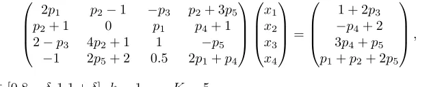
Example 3. Consider the following parametric interval linear system
2p1 p2−1 −p3 p2+ 3p5
p2+ 1 0 p1 p4+ 1
2−p3 4p2+ 1 1 −p5
−1 2p5+ 2 0.5 2p1+p4
x1
x2
x3
x4
=
1 + 2p3
−p4+ 2
3p4+p5
p1+p2+ 2p5
, (14)
wherepk∈[0.8−δ,1.1 +δ],k= 1, . . . , K= 5.
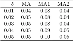
δ MA MA1 MA2 0.01 0.04 0.08 0.04 0.02 0.05 0.08 0.04 0.03 0.05 0.08 0.04 0.04 0.05 0.09 0.05 0.05 0.05 0.10 0.05
Table 2: Computational times (in seconds) for Example3.
Table 3 presents the obtained interval enclosures (the results are rounded to four decimal places). We can see from the table that for δ = 0.01,0.02,0.03 the standard version of the monotonicity approach produced the worst results. For δ = 0.01, the results of the MA1 method and the MA2 method coincide, whereas forδ= 0.02,0.03 the MA1 method is slightly better than the MA2 method. Forδ= 0.04 the advantage of MA1 over two other methods is significant, and forδ= 0.05 all the methods produced the same result. In order to show that it is important to take into account the dependencies in the system, we also provide in Table3the results of the Combinatorial Approach1(CA) method (see, e.g., [35]). The CA method produces
the interval hull solution of the corresponding interval linear system (obtained by neglecting the dependencies, i.e., by computing the interval extensions ofA(p) andb(p) overp).
Method δ= 0.01 δ= 0.02 δ= 0.03 δ= 0.04 δ= 0.05 MA [0.0334,1.0028] [−0.1152,1.1007] [−0.1723,1.1630] [−0.2345,1.2306] [−0.3027,1.3042] [0.5935,1.2378] [0.5702,1.2657] [0.5459,1.2949] [0.5204,1.3255] [0.4936,1.3577] [−1.5219,0.2774] [−1.7763,0.5719] [−1.8903,0.6998] [−2.0151,0.8405] [−2.1527,0.9963] [0.0831,0.6445] [0.0573,0.6655] [0.0302,0.6875] [0.0018,0.7107] [−0.0283,0.7358] MA1 [0.1115,0.9652] [0.0892,1.0065] [0.0669,1.0494] [0.0240,1.1238] [−0.3027,1.3042] [0.6537,1.2167] [0.6403,1.2403] [0.6265,1.2687] [0.5982,1.3077] [0.4936,1.3577] [−1.5219,0.2774] [−1.5982,0.3599] [−1.6787,0.4477] [−2.0151,0.8405] [−2.1527,0.9963] [0.1106,0.6090] [0.0898,0.6248] [0.0684,0.6408] [0.0381,0.6678] [−0.0283,0.7358] MA2 [0.1115,0.9652] [0.0773,1.0281] [0.0518,1.0749] [−0.2345,1.2306] [−0.3027,1.3042] [0.6440,1.2274] [0.6288,1.2532] [0.5459,1.2949] [0.5204,1.3255] [0.4936,1.3577] [−1.5219,0.2774] [−1.5982,0.3599] [−1.6787,0.4477] [−2.0151,0.8405] [−2.1527,0.9963] [0.1106,0.6090] [0.0838,0.6323] [0.0302,0.6875] [0.0018,0.7107] [−0.0283,0.7358] CA [−0.2814,1.3244] [−0.3381,1.3862] [−0.3965,1.4493] [−0.4561,1.5137] [−0.5170,1.5858] [0.5660,1.4164] [0.5491,1.4590] [0.5326,1.5032] [0.5164,1.5491] [0.4999,1.59688] [−2.1050,0.4641] [−2.2853,0.5750] [−2.48444,0.6921] [−2.7048,0.8156] [−2.9496,0.9456] [−0.0785,0.8710] [−0.1168,0.90483] [−0.15653,0.9390] [−0.1976,0.9738] [−0.2402,1.0092]
Table 3: Outer interval solutions (results are rounded to four decimal places) obtained using MA, MA1, MA2 and CA methods for Example3.
In order to assess the accuracy of the obtained enclosures, we use thesharpness measure[28], which is defined for two intervalsx, y(x⊆y) as
Os(x,y) =
1, y∆= 0,
0, x=∅, x∆
y∆, otherwise.
(15)
For interval vectors we take minimum and maximum values over all entries.
Table4presents the minimal and maximal values of the sharpness measureOs(x,y), where
x is the i-th component of computed interval enclosure and y is the i-th component of the inner estimation of the hull (IEH) solution produced by the evolutionary optimization (EO) method [33].
1
δ MA MA1 MA2 CA min-max min-max min-max min-max 0.01 0.77-0.87 0.77-1.00 0.77-0.99 0.52-0.66 0.02 0.63-0.86 0.76-1.00 0.76-0.96 0.51-0.66 0.03 0.62-0.85 0.75-0.99 0.75-0.94 0.50-0.65 0.04 0.60-0.84 0.60-0.95 0.60-0.84 0.49-0.65 0.05 0.59-0.83 0.59-0.83 0.59-0.83 0.47-0.65
Table 4: Comparison of accuracy of MA, MA1 and MA2 methods for Example3: minimal and maximal values of sharpness measure taken over all entries of solution vector.
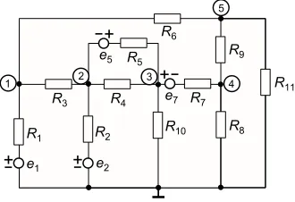
Example 4. Consider the parametric interval linear system (16), which occurs in worst-case tolerance analysis of linear AC (alternate current) electrical circuits [2, 6, 7, 40]. The circuit depicted in Fig. 2 (cf. Kolev [6]) has eleven branches and five nodes. The goal here is to find bounds for the node voltagesV1, . . . , V5. The parameters of the model have the following
nominal values:
e1=e2= 100V, e5=e7= 10V,
Zj=Rj+iXj ∈C, Rj= 100Ω, Xj=ωLj− 1 ωCj
, j= 1, . . . ,11,
ω= 50, X1,2,5,7=ωL1,2,5,7= 20, X3=ωL3= 30,
X4=− 1
ωC4
=−300, X10=− 1
ωC10
=−400, X6,8,9,11= 0.
The worst-case tolerance analysis leads to a complex parametric interval linear system [7,27]
1
Z1 +
1
Z3 +
1
Z6 −
1
Z3 0
− 1
Z3
1
Z2 +
1
Z3 +
1
Z4 +
1
Z5 −
1
Z4 −
1
Z5 0 −Z14 −Z15 Z14 +Z15 +Z17 +Z110
0 0 −Z17
− 1
Z6 0 0
(16)
0 − 1
Z6
0 0
−1
Z7 0
1
Z7 +
1
Z8 +
1
Z9 −
1
Z9 −Z19 Z16+Z19 +Z111
V1 V2 V3 V4 V5 = e1 Z1 e2 Z2 −
e5 Z5 e5 Z5 +
e7 Z7 −e7
Z7 0 , where
Z1=Z2=Z5=Z7= 100 +i20, Z3= 100 +i30, Z4= 100−i300,
Z6=Z8=Z9=Z11= 100, Z10= 100−i400.
We putpj = 1/Zjand we solve the system with tolerances±5%,±10%,±15% and±20%. The computational times (in seconds) are presented in Table5. As can be seen, the MA and MA2 methods have similar computational times, whereas the MA1 method, as expected, is much more expensive.
R1
e1
+
+ +
+
2
1 3 4
5
R3
R2
R10 R8
R11 R9
R6
R7 R5
R4
e2
e5
e7
Figure 2: (Example4) Linear electrical circuit with five nodes and eleven branches.
Uncertainty MA MA1 MA2
5% 0.8 2.1 0.7
10% 1.1 2.6 1.0
15% 1.5 3.5 1.4
20% 2.5 5.6 2.5
Table 5: Computational times (in seconds) for Example4.
Uncertainty MA MA1 MA2
min-max min-max min-max 5% 0.96-0.99 0.99-1.00 0.99-1.00 10% 0.80-0.96 0.83-0.99 0.82-0.98 15% 0.46-0.81 0.53-0.92 0.53-0.88 20% 0.28-0.54 0.28-0.54 0.28-0.54
Table 6: Comparison of accuracy MA, MA1 and MA2 methods for Example 4: minimal and maximal values of sharpness measure taken over all entries of interval solution vector.
solution produced by the EO method. Additionally, the interval solution vector obtained for 5% uncertainty is provided in Table7.
As can be seen from Table6, also in this case the MA1 and MA2 methods outperformed the standard approach. The MA2 method produced slightly worse results than the MA1 method, however it turned out to be more efficient.
Voltage EO MA2
V1 [64.8265,69.4151] +i[−7.4030,−5.6879] [64.8259,69.4158] +i[−7.4083,−5.6817]
V2 [69.0870,73.5915] +i[−8.7003,−6.4356] [69.0867,73.5926] +i[−8.7089,−6.4305]
V3 [53.3405,58.9868] +i[−13.0941,−9.7543] [53.3347,58.9913] +i[−13.1005,−9.7474]
V4 [22.9180,27.2849] +i[−7.4055,−5.7220] [22.9166,27.2855] +i[−7.4076,−5.7193]
V5 [28.5406,33.0201] +i[−5.0545,−3.7151] [28.5401,33.0209] +i[−5.0554,−3.7130]
Table 7: Results (rounded to four decimal places) of EO and MA2 methods for 5% uncertainty; Example4.
Figure 3: (Example5) Planar frame (left) and its fundamental system of internal parameters (right) (cf. [17]).
moments (see Fig. 3 (right)) and three canonical equations linking bending moments with material properties of the beams. Similarly as in [17], we assume here that all beams have the same Young modulusE, but momentum of inertiaJ of beam cross-sections are related by the formulaJ12 =J23 = 1.5J24. Taking this into account, the combination of the equilibrium
and canonical equations yields the following system of linear equations for reaction forces and bending moments:
2l12 l12 0 0 0 0 0 0
l12 2l12+ 2l23 −2l23 0 0 0 0 0
0 −2l23 3l24+ 2l23 0 0 0 0 0
0 0 0 0 0 0 1 1
0 0 0 1 1 1 0 0
−1 0 0 0 l12 l12+l24 0 l23
−1 1 0 −l12 0 0 0 0
0 0 −1 0 0 l24 0 0
M1 M21 M24
Ry1 Ry3 Ry4 Rx 1 Rx 3 = 0 0 −3 8ql 3 24 0 ql24
ql24 l12+12l24
0 1 2ql 2 24
The lengths of the beams and the load are considered to be uncertain2and vary within intervals:
l12, l24∈[1−δ,1 +δ],l23∈0.75[1−δ,1 +δ],q∈10[1−δ,1 +δ]. The parameters of the frame
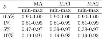
are given as dimensionless numbers; however it is assumed that the values of the parameters are physically realistic when endowed with appropriate units (cf. [17]). We solve the problem forδ= 0.5%,1%,5%,10%. The computational times are provided in Table 8.
Table 9 presents the accuracy of the obtained interval enclosures. Similarly as in the previous examples, we compare outer interval enclosures with inner estimation of the hull solution produced by the EO method. Additionally, the results of the EO and MA2 methods forδ= 1% are provided in Table10.
δ MA MA1 MA2 0.5% 0.11 0.17 0.09 1% 0.11 0.17 0.09 5% 0.13 0.17 0.10 10% 0.14 0.19 0.12
Table 8: Computational times (in seconds) for Example5.
2
δ MA MA1 MA2 min-max min-max min-max 0.5% 0.90-1.00 0.90-1.00 0.90-1.00 1% 0.81-0.99 0.81-0.99 0.81-0.99 5% 0.47-0.97 0.39-0.97 0.39-0.97 10% 0.19-0.91 0.19-0.93 0.19-0.93
Table 9: Comparison of outer interval solutions obtained using MA, MA1 and MA2 methods for Example5: minimal and maximal values of sharpness measure taken over all entries of solution vector.
EO MA2
M1 [0.2397,0.2607] [0.2395,0.2607]
M21 [−0.5213,−0.4793] [−0.5213,−0.4790]
M24 [−1.0344,−0.9664] [−1.0344,−0.9657]
Ry
1 [−0.7899,−0.7119] [−0.7899,−0.7113]
Ry
3 [6.5905,6.9126] [6.5872,6.9150]
Ry
4 [3.9204,4.0804] [3.9179,4.0811]
Rx
1 [−0.7021,−0.6328] [−0.7085,−0.6227]
Rx
3 [0.6328,0.7021] [0.6227,0.7085]
Table 10: Results (rounded to four decimal places) of EO and MA2 methods for δ = 1%; Example5
4
Conclusion
We have proposed in this work two modifications of the monotonicity approach for solving parametric interval linear systems. Based on the obtained results we can conclude that, generally, the MA2 method (which is based on using the p-solution) is most recommended. It produces similar results as the MA1 methods, whereas it is computationally much more efficient. In our future work we will try to employ parallel techniques in order to decrease the computational time. Also we will try to combine monotonicity approach with some other methods for solving parametric interval linear systems.
5
Acknowledgments
We would like to thank the reviewers for their time spent on reviewing our manuscript and for their insightful comments that helped us to improve this paper.
M. Hlad´ık was supported by the Czech Science Foundation Grant P403-18-04735S.
References
[1] Ramil R. Akhmerov. Interval-Affine Gaussian Algorithm for Constrained Systems. Reliable Computing, 11:323–341, 2005.
[2] Alexander Dreyer.Interval analysis of analog circuits with component tolerances. Ph.d. thesis, TU Kaiserslautern, Aachen, Germany, 2005.
[3] Hassan El-Owny. Outer interval solution of linear systems with parametric interval data.
[4] Milan Hlad´ık. Description of symmetric and skew-symmetric solution set. SIAM J. Matrix Anal. Appl., 30(2):509–521, 2008.
[5] Milan Hlad´ık. Enclosures for the solution set of parametric interval linear systems. Int. J. Appl. Math. Comput. Sci., 22(3):561–574, 2012.
[6] Lubomir Kolev. Interval Methods for Circuit Analysis. World Scientific, 1993.
[7] Lubomir V. Kolev. Worst-case tolerance analysis of linear DC and AC electric circuits. IEEE Trans. Circuits Syst. I: Fundam. Theory Appl., 49(12):1693–1701, 2002.
[8] Lubomir V. Kolev. A method for outer interval solution of linear parametric systems. Reliable Computing, 10(3):227–239, 2004.
[9] Lubomir V. Kolev. Solving Linear Systems Whose Elements Are Non-linear Functions of Intervals.
Reliable Computing, 10(3):227–239, 2004.
[10] Lubomir V. Kolev. Improvement of a direct method for outer solution of linear parametric systems.
Reliable Computing, 12(3):193–202, 2006.
[11] Lubomir V. Kolev. Componentwise determination of the interval hull solution for linear interval parameter systems.Reliable Computing, 20(1):1–24, 2014.
[12] Lubomir V. Kolev. Parameterized solution of linear interval parametric systems. Appl. Math. Comput., 246:229–246, 2014.
[13] Lubomir V. Kolev. Parameterized solution of linear interval parametric systems. Applied Mathematics and Computation, 246:229–246, 2014.
[14] Lubomir V. Kolev. Iterative algorithms for determining a p-solution of linear interval parametric systems. In Advanced Aspects of Theoretical Electrical Engineering, Sofia, Bulgaria, pages 15.09–16.09, 2016.
[15] Vladik Kreinovich, Anatoly Lakeyev, Jiˇri Rohn, and P.T. Kahl. Computational Complexity and Feasibility of Data Processing and Interval Computations. Kluwer, Dordrecht, 1998.
[16] Vladik Kreinovich and Anatoly V. Lakeyev. Linear interval equations: Computing enclosures with bounded relative or absolute overestimation is NP-hard.Reliab. Comput., 2(4):341–350, 1996. [17] Zenon Kulpa, Andrzej Pownuk, and Iwona Skalna. Analysis of Linear Mechanical Structures with
Uncertainties by Mean of Interval Methods. CAMES, 5:443–477, 1998.
[18] G¨unter Mayer. An Oettli–Prager-like theorem for the symmetric solution set and for related solution sets.SIAM J. Matrix Anal. Appl., 33(3):979–999, 2012.
[19] G¨unter Mayer. Three short descriptions of the symmetric and of the skew-symmetric solution set.
Linear Algebra Appl., 475:73–79, 2015.
[20] Svatopluk Poljak and Jiˇr´ı Rohn. Checking robust nonsingularity is NP-hard.Math. Control Signals Syst., 6(1):1–9, 1993.
[21] Evgenija D. Popova. On the solution of parametrised linear systems. In W. Kr¨amer and J.W. von Gudenberg, editors,Scientific Computing, Validated Numerics, Interval Methods, pages 127–138, London, 2001. Kluwer.
[22] Evgenija D. Popova. Computer-assisted proofs in solving linear parametric problems. In12th GAMM/IMACS International Symposium on Scientific Computing, Computer Arithmetic and Validated Numerics, SCAN 2006, pages 35–35, Duisburg, Germany, 2006.
[23] Evgenija D. Popova. Solving linear systems whose input data are rational functions of interval parameters. LNCS, 4310:345–352, 2007.
[24] Evgenija D. Popova. Explicit characterization of a class of parametric solution sets. Comptes Rendus de L’Academie Bulgare des Sciences, 62(10):1207–1216, 2009.
[25] Evgenija D. Popova. Improved enclosure for some parametric solution sets with linear shape.
Comput. Math. Appl., 68(9):994–1005, 2014.
[26] Evgenija D. Popova. Solvability of parametric interval linear systems of equations and inequalities.
[27] Evgenija D. Popova, Lubomir Kolev, and Walter Kr¨amer. A Solver for Complex-Valued Parametric Linear Systems. Serdica Journal of Computing, 4(1), 2010.
[28] Evgenija D. Popova and Walter Kr¨amer. Inner and outer bounds for the solution set of parametric linear systems. Journal of Computational and Applied Mathematics, 199(2):310–316, 2007. [29] Jiˇr´ı Rohn. A method for handling dependent data in interval linear systems. Technical Report
911, Institute of Computer Science, Academy of Sciences of the Czech Republic, Prague, 2004.
https://asepactivenode.lib.cas.cz/arl-cav/en/contapp/?repo=crepo1&key=20925094170. [30] Siegfried M. Rump. Verification methods for dense and sparse systems of equations. In
J. Herzberger, editor,Topics in Validated Computations, pages 63–136, Amsterdam, 1994. Elsevier. [31] Siegfried M. Rump. Verification methods: Rigorous results using floating-point arithmetic. Acta
Numerica, 19:287–449, 2010.
[32] Iwona Skalna. A method for outer interval solution of systems of linear equations depending linearly on interval parameters. Reliable Computing, 12(2):107–120, 2006.
[33] Iwona Skalna. Evolutionary optimization method for approximating the solution set hull of parametric linear systems. Lecture Notes in Computer Science, 4310:361–368, 2007.
[34] Iwona Skalna. On checking the monotonicity of parametric interval solution of linear structural systems. Lecture Notes in Computer Science, 4967:1400–1409, 2008.
[35] Iwona Skalna. A global optimization method for solving parametric linear systems whose input data are rational functions of interval parameters. Lecture Notes in Computer Science, 6068:475–484, 2010.
[36] Iwona Skalna. Enclosure for the Solution Set of Parametric Linear Systems with Non-affine Dependencies. In Roman Wyrzykowski, Jack Dongarra, Konrad Karczewski, and Jerzy Wa´sniewski, editors,Parallel Processing and Applied Mathematics, volume 7204 ofLNCS, pages 513–522. Springer, 2012.
[37] Iwona Skalna. Parametric Interval Algebraic Systems. Springer International, 2018.
[38] Iwona Skalna and Jerzy Duda. A study on vectorisation and paralellisation of the monotonicity approach. In R. Wyrzykowski et al., editor,Parallel Processing and Applied Mathematics, volume 9574 ofLNCS, pages 455–463. Springer, 2016.
[39] Iwona Skalna and Milan Hlad´ık. A new method for computing ap-solution to parametric interval linear systems with affine-linear and nonlinear dependencies.BIT Numer. Math., 57(4):1109–1136, 2017.

![Figure 3: (Example 5(right) (cf. [) Planar frame (left) and its fundamental system of internal parameters17]).](https://thumb-us.123doks.com/thumbv2/123dok_us/8878226.1818130/11.612.102.514.344.442/figure-example-right-planar-frame-fundamental-internal-parameters.webp)