ISSN: 2008-6822 (electronic)
http://www.ijnaa.semnan.ac.ir
A modified LLL Algorithm for
Change of Ordering of Gr¨
obner Basis
M. Borujenia, A. Basiria,∗, S. Rahmanya, A. H. Borzabadia
aSchool of Mathematics and Computer Science, Damghan University, Damghan, Iran
Abstract
In this paper, a modified version of LLL algorithm, which is a an algorithm with output-sensitive complexity, is presented to convert a given Gr¨obner basis with respect to a specific order of a poly-nomial ideal I in arbitrary dimensions to a Gr¨obner basis of I with respect to another term order. Also a comparison with the FGLM conversion and Buchberger method is considered.
Keywords: Gr¨obner Basis, LLL Algorithm, Reduced Lattice Basis.
2010 MSC: Primary 13P10 ; Secondary 16G30.
1. Introduction
One of the main tools for solving nonlinear systems is the computation of Gr¨obner bases. Buch-berger algorithm [3] computes a Gr¨obner basis for a polynomial idealI with respect to an admissible term ordering<. There are different algorithms like F4 and F5 which were presented by Faugere in [5] and [6], to improve Buchberger algorithm. Runtime and memory requirements for computing a Gr¨obner basis is heavily dependendent on the term ordering <. The lexicographic term orders are enable to eliminate some variables and hence they can be used for solving polynomial systems and unfortunately, computing the consumes Gr¨obner basis wrt lexicographic order consumes a lot of time and memory than other orders. Changing of ordering can be given rise to overcome this problem. Among the all term orders, the total degree term order is one of the best orders, that the computing Gr¨obner basis respect to it, can be done by consuming reasonable time and memory and this is a intensive incentive for computing a total degree Gr¨obner basis and converting it to a lexicographic Gr¨obner basis. When the ideal is zero-dimensional, The algorithms presented in [7, 8] are efficients for converting the ordering of Gr¨obner basis. The aim of this paper is to introduce an algorithm to convert the ordering of a Gr¨obner basis when the dimension of ideal is positive.
∗Corresponding author
Email addresses: [email protected] (M. Borujeni ),[email protected](A. Basiri ),[email protected]
(S. Rahmany),[email protected] (A. H. Borzabadi)
The idea of using LLL algorithm was first proposed by Basiri and Faugere [1], for change ordering of Gr¨obner basis in polynomial ring with two variables. In this paper, we tend to introduce an extension of this idea, considering a new modified LLL algorithm for conversion a Gr¨obner basis of an ideal with respect to <old into a Gr¨obner basis with respect to <new, in polynomial rings with n
variables, wheren ≥2.
The rest of the paper is organized as follows. Section 2 is devoted to present some requirement perliminaries. In Section 3, modified LLL algorithm along with its correctness and termination are described. Experimental results and a comparision with the FGLM and Buchberger methods are shown in Section 4.
2. Perliminaries and Definitions
In this section some requirement concepts and properties of Gr¨obner basis and lattice basis will be introduced. We refer to [4, 2] for basic facts and notations.
Let K[x] be a polynomial ring in variables x1,· · · , xn over an arbitrary field K and I be an
ideal. The ideal generated by a set of polynomials {g1,· · · , gm} ⊂K[x] is denoted by hg1,· · · , gmi.
Considering an admissible ordering <, we denote by lt(f) the leading term of a polynomial f. An element f ∈ K[x] is reduced by a Gr¨obner basis G if no element g ∈ G has a leading term that divides some terms of f. A Gr¨obner basis Gis reduced if each g ∈G is reduced byG− {g}.
Theorem 2.1. Let n, d1,· · · , dn∈IN andwbe not more thand1d2· · ·dn−1, then there exist unique numbers 06wi 6di−1, such that
w=w1d2d3· · ·dn+w2d3· · ·dn+· · ·+wn−2dn−1dn+wn−1dn+wn.
Proof . The proof is by induction on n. For n = 1, let w1 = w. Suppose d1,· · · , dn ∈ IN and
0 6 w 6 d1d2· · ·dn−1. By division algorithm, w = w1d2· · ·dn+r, where 0 6 r 6 d2· · ·dn −1
and w1 6 d1 −1, because w1 > d1 is contrary to w 6 d1d2· · ·dn−1. By induction assumption,
r=w2d3· · ·dn+· · ·+wn−1dn+wn, where 06wi 6di−1. Thus
w=w1d2· · ·dn+w2d3· · ·dn+· · ·+wn−1dn+wn.
Suppose that 06w˜i 6di−1, for 16i6n, satisfy in properties of the theorem. So
n−1 X
i=2 ˜
widi+1· · ·dn−1+ ˜wn6d2d3· · ·dn−1.
By uniqueness of r and w1 the proof is complete.
Let (G={g1,· · · , gm}, <) be a reduced Gr¨obner basis forI and
αi = max{degxi(gj)| 16j 6m},
and alsoc= (α1+ 1)· · ·(αn−1+ 1).
By Theorem 2.1, for 06d6c, there exist unique numbers 06sd,j, 16j 6n−1, such that
d= 1 +sd,n−1+sd,n−2(αn−1+ 1) +· · ·+sd,1(α2+ 1)· · ·(αn−1 + 1).
Let sd = (sd,1,· · · , sd,n−1) and sG = {s1,· · · , sc} ⊂ IN0n−1. For f ∈ K[x] we define α(f) = the xβ1
1 · · ·x
βn−1
n−1 , where lt(f) =x
β1
Definition 2.2. Let(G={g1,· · · , gm}, <)be a reduced Gr¨obner basis forIandlt(gi) =x αi,1 1 · · ·x
αi,n
n ,
for 1 6 i 6 m. We can consider a change in the indices such that, α(gi) < α(gi+1). For integer
numbers di ≥degxi(lt(gj)), i= 1,· · · , n−1, define
BG ={xt11· · ·x
tn−1
n−1gi |tj 6dj−αi,j, 16i6m, 16j 6n−1},
A ={xt1 1 · · ·x
tn−1
n−1gi ∈/ G| ∃ 16j 6m, i < j, s.t. α(xk11· · ·x
kn−1
n−1gj) = α(xt11· · ·x
tn−1
n−1gi)}
Bs(G) =BG−A.
We denote by Ms(G) the K[xn]-submodule of K[x] generated by Bs(G) which is called s-th K[xn] -module associated to idealI with respect to<. In this case,Bs(G)is calleds-th basis ofK[xn]-module associated to ideal I, with respect to <.
Let ˜b1,· · ·,˜bl be vectors in K[xn]c which are linearly independent over K[xn], where l and c are
positive integers and l6c. The latticeL⊂K[xn] c
of rankl spanned by ˜b1,· · · ,˜bl is defined as
L=
l
X
i=1
K[xn]˜bi ={ l
X
i=1
λi˜bi| λi ∈K[xn], 16i6l}.
Consider the natural mapping from K[xn]c to K[x], which corresponds the vector ˜v = (v1,· · · , vc)
to the polynomial v =Pc
j=1vjx1sj,1· · ·xn−1sj,n−1. Under this mapping, the lattice L⊂K[xn] c
corre-sponding to theK[xn]−submoduleM(L) ofK[x] is denoted by
M(L) = {v =
c
X
j=1
vjx1sj,1· · ·xn−1sj,n−1| v˜= (v1,· · · , vc)∈L}.
Letb1,· · ·, blbe a basis for theK[xn]−submoduleM(L) ofK[x] and let ˜b1,· · · ,˜bl be the
correspond-ing basis for the latticeL.We denote byB = (bi,jx1sj,1· · ·xn−1sj,n−1) the l×cmatrix wherebi,j is the
coefficient of x1sj,1· · ·xn−1sj,n−1 in the polynomial bi =
Pc
j=1bi,jx1sj,1· · ·xn−1sj,n−1. Then we define determinant d(M(L)) of M(L) to be the maximum of the determinant of l×l sub-matrices of B with respect to<, and the determinant d(L) ofL to be the determinantd(M(L)) of M(L). Finally, the orthogonality defect OD(˜b1,· · · ,˜bl) of the basis ˜b1,· · · ,˜bl for the lattice L with respect to <, is
defined as
lt(b1)· · ·lt(bl)−lt(d(L)).
Definition 2.3. The basis˜b1,· · · ,˜bl is called reduced if OD(˜b1,· · · ,˜bl) = 0.
For 1 6 i 6 l, ith successive minimum (non-unique) of M(L) with respect to < is a minimum element mi of M(L), such that mi does not belong to the K[xn] submodule of M(L), generated by
m1,· · · , mi−1.
Proposition 2.4. Let b˜1,· · · ,b˜l be a reduced basis for a lattice L ⊂ K[xn]c of rank l 6 c, which is ordered in such a way that bi 6 bj for 1 6 i < j 6 l. Then for 1 6 i 6 l, bi is an ith successive minimum of M(L) with respect to <.
Proposition 2.5. Let˜b1,· · · ,˜bl be a basis for lattice L⊂K[xn]c of rank l6c. If the coordinates of the vectors b˜1,· · · ,b˜l can be permuted so that they satisfy
bi 6bj, for 16i < j 6l,
bi,j < bi,i >bi,k, for 16i < j 6l, i < k≤c, then the basis b˜1,· · · ,˜bl is reduced.
Proof . See [11].
Theorem 2.6. Let (G={g1,· · · , gm}, <) be a reduced Gr¨obner basis for I, d1,· · · , dn−1 be positive
integer numbers such that di ≥degxi(lt(gj)) for 16i6n−1, 16j 6m, and
Is(G) = {f ∈I |α(f) = xk11· · ·x
kn−1
n−1, k1 6d1,· · · , kn−1 6dn−1},
then Is(G) =Ms(G).
Proof . Because Bs(G) ⊂ Is(G) then Ms(G) ⊂ Is(G). If Ms(G) 6= Is(G), let h be the minimum
polynomials (with respect to <) in Is which does not belong to Ms(G). Let lt(h) = x β1
1 · · ·xβnn
and i0 = max{i | lt(gi)|lt(h)}, then αi0,j 6 βj, for 1 6 j 6 n. We have βj 6 dj for 1 6 j 6 n, because h∈Is(G), thus βj −αi0,j 6dj −αi0,j. Let b=x
β1−αi0,1 1 · · ·x
βn−1−αi0,n−1
n−1 gi0. Choosingi0 and b ∈ Bs(G), we put ˜h = h− HCHC((hb))x
βn−αi0,n
n b. We claim that ˜h does not belong to Ms(G), because
otherwise h = ˜h+ HCHC((hb))xβn−αi0,n
n b is a member of Ms(G) which is a contradiction with the choice
of h. On the other hand, lt(HCHC((hb))xβn−αi0,n
n b) = xβ11· · ·xnβn = lt(h) and so lt(˜h) < lt(h). Therefore,
˜
h < hthat is a contradiction with the choice of h. Hence Ms(G) = Is(G).
3. Modified LLL Algorithm
In this section we present a new version of LLL algorithm [10], which computes a Gr¨obner basis for term order <new from the Gobner basis corresponding to term order <old) in K[x] and in the
end, termination and correctness of the given algorithm will be proved. This algorithm contains two major steps: initialization step and main steps. In initialization step, a basis Bs(Gold) is produced
where the K[xn]-module generated by it, includes a Gr¨obner basis with respect to <new. In main
steps, first a matrix by the elements of Bs(Gold) is created and then using linear algebra techniques,
this matrix is converted to a new matrix, where its orthogonality default is equal to zero. It will be justified that the rows of last matrix forms a Gr¨obner basis with respect to<new.
LLL Algorithm. Initialization step
Consider (Gold={g1,· · · , gm}, <old) as a reduced Gr¨obner basis for I, <new, and
di, i= 1· · · , n−1, as positive integers sufficiently large.
Set {b1,· · · , bl}:=Bs(Gold), and k:= 0.
Main steps
1. Choose i0 ∈ {k+ 1,· · · , l} s.t. bi0 = min<new{bi |k+ 16i6l}and swap(˜bk+1,˜bi0). 2. Choose j ∈ {1,· · · , c} s.t. HTnew(bk+1) = HTnew(bk+1,j).
3. Ifj 6k set ˜t := ˜bk+1−
HCnew(bk+1)
HCnew(aj) x
deg(˜bk+1,j)−deg(˜aj,j)
n ˜aj, otherwise, ˜t := ˜bk+1. 4. IfHTnew(t) = HTnew(bk+1) then ˜ak+1 := ˜t. Permute (k+ 1,· · ·, n) such that HTnew(ak+1,k+1) =HTnew(ak+1).
k :=k+ 1 and if k=l stop. Otherwise go to step 1.
5. IfHTnew(t)<new HTnew(bk+1) thenp:= max{06s6k |as <new t}and for
Theorem 3.1. LLL algorithm computes a Gr¨obner basisGnewinK[x], such thatId(Gold) = Id(Gnew).
Proof . Letd1,· · · , dn−1 be a positive integer such that
di >max{degxi(lt(g)), degxi(lt(h)) f or g∈Gold and h∈G}
for 16i6n−1, where Gis a Gr¨obner basis for I with respect to <new, then G⊂Is(Gold) and by
Theorem 2.6,Ms(Gold)⊆Is(Gold). Therefore, Bs(Gold) is a Gr¨obner basis forI with respect to<old,
where K[xn]-module generated by it, includes a Gr¨obner basis with respect to <new.
Termination: There are finite numbers of passages through step 4 because k is increased by 1.
Also there are finite numbers of passages through step 5, because
lt(a1)· · ·lt(ak)lt(bk+1)· · ·lt(bn)
becomes smaller than previous step and stays unchanged in the step 4. Hence, the number of passages in the main steps are finite and algorithm terminates when k=l.
Correctness: Clearly, Bs(Gold) and {a1,· · · , al} generate the same K[xn] submodule M of K[x].
By Theorem 2.6, M = Is(Gold). On the other hand, by Proposition 2.5, {e˜a1,· · · ,˜al} is a reduced
basis for the lattice Lwith basis {b1,· · · , bl}, because the following invariants are valid before steps
1 and 4
ai 6aj , for 16i < j 6k,
ak 6bj, for k < j6l,
ai,j < ai,i > ai,r, f or 16j < i6k and i < r6c.
Hence by Proposition 2.4, ai is ith successive minimum of M and lt(ai) < lt(ai+1), (otherwise lt(ai) = lt(ai+1), and then a
0
=ai+1−ai ∈M and lt(a
0
)<lt(ai+1) imply that a
0
is dependent upon the rowsa1,· · · , ai, so ai+1 =a
0
+ai is also dependent witha1,· · ·, ai, which is a contradiction with
the choice of ai+1). Now, let g be a polynomial in Is(Gold) = M, then there are λ1,· · · , λl ∈ K[xn]
such that
g =
l
X
j=1 λjaj.
But for 1 6 i < j 6 l, lt(λiai) 6= lt(λjaj), because otherwise there are ti, tj such that lt(λiai) =
xtinlt(ai) and lt(λjaj) = x tj
nlt(aj), but lt(ai)<lt(aj) impliesti > tj (ifti < tj thenxtinlt(ai)< x tj nlt(aj),
and ifti =tj then lt(ai) = lt(aj)) and hencea
0
=xtin−tjai−aj ∈M and lt(a
0
)<lt(aj) which impliesa
0
is dependent upona1,· · · , aj−1, soaj =x ti−tj
n ai−a
0
depends ona1,· · · , aj−1 which is a contradiction with the choice of aj. Finally, there is a unique 1 6j 6l such that lt(g) = lt(λjaj), so lt(aj)|lt(g).
On the other hand, G is a Gr¨obner basis and for any polynomial f ∈ I, there exists g ∈ G ⊂ M such that lt(g)|lt(f) and thereupon lt(aj)|lt(f) which reveals that{a1,· · · , al}is a Gr¨obner basis for
I with respect to<new.
4. Experimental Results
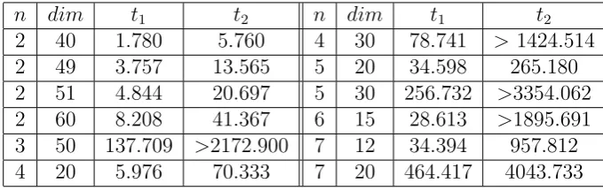
To demonstrate the efficiency of the presented algorithm in previous section, a Gr¨obner basis with respect to DRL order in case of general andnvariables, which is Gr¨obner basis generated by random polynomials, is considered. Results of implementing this modified algorithm and compare it with FGLM algorithm and Gr¨obner basis algorithm available in Maple can be observed in Tables 1 and 2, respectively. Note, here we didn’t compute Bs(Gold), because there is not any gap between α(gi)
notations is used in Tables: n is the number of variables,D= max{α1,· · · , αn}is degree of Gr¨obner
basis , dim is dimension of K-vector space KI[x], Nm is the number of multiplications for algorithm,
t1 is LLL algorithm execution time andt2 is Gr¨obner basis algorithm (available in Maple) execution time.
n D dim n.dim3 N
m n D dim n.dim3 Nm
2 3 5 250 25 3 4 20 24000 18323
2 4 10 2000 329 3 5 30 81000 120428
2 5 15 6750 1105 4 2 4 256 162
2 6 20 16000 2826 4 3 8 2048 1338
3 3 5 375 108 5 2 3 135 52
3 3 10 3000 1590 5 3 10 5000 8563
Table 1: The results of comparison between LLL and FGLM algorithms(DRL to Lex)
n dim t1 t2 n dim t1 t2 2 40 1.780 5.760 4 30 78.741 > 1424.514
2 49 3.757 13.565 5 20 34.598 265.180
2 51 4.844 20.697 5 30 256.732 >3354.062 2 60 8.208 41.367 6 15 28.613 >1895.691 3 50 137.709 >2172.900 7 12 34.394 957.812
4 20 5.976 70.333 7 20 464.417 4043.733
Table 2: The results of comparison of LLL algorithm with Gr¨obner basis algorithm (available in Maple)(DRL to Lex)
5. Conclusion
The modified version of LLL algorithm converts a Gr¨obner basis of an ideal with respect to an arbitrary ordering into a Gr¨obner basis with respect to another desired ordering. Although in some cases, complexity of FGLM algorithm is less than LLL algorithm complexity, but an important feature of LLL algorithm lies in the fact that it can compute Gr¨obner basis for ideals of positive dimension while FGLM algorithm can compute it only for ideals of zero dimension.
Acknowledgments
The authors would like to thank Damghan university for supporting this research.
References
[1] A. Basiri and J.-C. Faug`ere. Changing the ordering of Grbner bases with LLL: Case of two variables. In J. R. Sendra, editor,Proceedings of ISSAC, pages 23–29. ACM Press, August 2003.
[2] T. Becker and V. Weispfenning. Gr¨obner bases. Springer-Verlag, NewYork-Berlin-Heidelberg, 1993.
[4] D. A. Cox, J. Little, and D. O’Shea. Ideals, Varieties, and Algorithms: An Introduction to Computational Algebraic Geometry and Commutative Algebra, 3/e (Undergraduate Texts in Mathematics). Springer-Verlag New York, Inc., Secaucus, NJ, USA, 2007.
[5] J.-C. Faug`ere. A new efficient algorithm for computing Gr¨obner bases (F4).Journal of Pure and Applied Algebra, 139(1–3):61–88, June 1999.
[6] J.-C. Faug`ere. A new efficient algorithm for computing Grbner bases without reduction to zero (F5). In T. Mora, editor,Proceedings of ISSAC, pages 75–83. ACM Press, July 2002.
[7] J.-C. Faug`ere, P. Gianni, D. Lazard, and T. Mora. Efficient computation of zero-dimensional Gr¨obner bases by change of ordering. Journal of Symbolic Computation, 16:329–344, 1993.
[8] J.-C. Faugre and C. Mou. Fast Algorithm for Change of Ordering of Zero-dimensional Gr¨obner Bases with Sparse Multiplication Matrices. InProceedings of the 36th international symposium on Symbolic and algebraic computation, ISSAC ’11, pages 115–122, New York, NY, USA, 2011. ACM.
[9] A.-K. Lenstra. Factoring multivariate polynomials over finite fields. Journal of Computer and System Sciences, 30(2), 1985.
[10] A.-K. Lenstra, H.-W. Lenstra, and L. Lov´asz. Factoring polynomials with rational coefficients. Math. Ann., 261:515–534, 1982.