LINKAGE BETWEEN LABOUR, OUTPUT AND
WAGES IN INDIAN MANUFACTURING
SECTOR- AN ECONOMETRIC ANALYSIS
Abstract: This study aims to investigate thelinkage between labour, output and wages in Indian manufacturing sector. More specifically, the study aims to investigate theshort-run causality and the long-run relationship between wages, growth and labour in Indian manufacturing sector. In addition, this study also tests the convergence speed or the error correction towards the equilibrium using vector error correction model. By investigating annual time series data set of a number of labourers employed, real wages and gross domestic product growth in Indian manufacturing sector, the empirical results of econometric analysis confirm the bilateral causality between number of labourers and gross domestic product growth, real wages and gross domestic product growth and real wages and number of labourers. Further, one Co-integrating equation has been found between all the variables of the study. The Coefficient of the error-correction term of overall model is statistically significant, with the speed of convergence to equilibrium equal to 20.9 percent. The stability of the system is confirmed and speed of adjustment is found to be very rapid.
Keywords: Gross domestic product; real wages; number of labourers; Indian Manufacturing; econometric analysis
1. INTRODUCTION
Liberalization measures adopted by India have focused on economic recovery of the country through augmenting employment opportunities with continuous additions to the labour force. In India, agriculture is still the largest source of employment whereas the contribution of industry in this regard is least [1]. There is a huge disparity between output and employment in the agriculture sector. The sector contributes about 14.4 percent of GDP but employs about 58.2 percent of the total workforce [2]. Indian industrial labour market has dualistic nature where both organized and unorganized sector co-exist. Laws related to industrial labour apply only to organized sector. However, unorganized sector finds no binding from the labour legislation of the country [3] [4] [5]. The Indian manufacturing sector has shown a remarkable growth, however, it is still lagging behind the manufacturing sectors of other East Asian countries in terms of contribution towards employment, generation of output and wage policies. The contribution of Indian manufacturing sector to the GDP of the country was around 16 percent in the 2006-2007 fiscal, whereas in China it was around 37 percent in the relevant year. Despite growth over the years, the growth in India's manufacturing sector is regarded as ‘jobless growth' because the sector shares only 13 percent of the total employment of
Nufzil Altaf
Research Scholar, School of Business Studies, Central University of Kashmir, J&K (India)
the country, with a contribution to GDP equal to 26.13 [6]. The sector has not been able to shift the focus of people from agriculture to industries [1].
The organized manufacturing sector of India has shown unsatisfactory performance in most states and has failed to provide adequate employment [7]. Presently 13 percent of the total employment is provided by manufacturing sector which is below than its true potential. To increase employment potential in manufacturing industries, it is imperative to focus on building more industries and improving the condition of present industries [8]. Moving towards economic recovery and growth, a country needs to make changes in its macroeconomic policies that can lead to a rise in labour employment, output and regulated wages [9].
It is widely recognized in the economics literature, that labour markets are central to an economic progress of developing nations since employment is directly related to the persistent poverty. However, due to the failure of labour markets in developing nations to create jobs agriculture still remains a dominant occupation for deriving livelihood in emerging economies. One of the challenges faced by emerging markets is gender disparities in employment. Women face barriers to accessing jobs informal sector however they over-represent the informal sector of the economy. Women in emerging markets are more of domestic workers rather than workers of a formal economy. There are a number of factors that lead to the poor representation of women in the formal economy, like, inadequate government support, educational levels, traditional beliefs and norms etc. Another concern for emerging markets is the growing population rates and lower employment opportunities [10]. The alarming figures of International labour organization (ILO) amplify that approximately 75 million people of age group 15-24 are unemployed, which is again a major concern for policy makers in developing nations [11]. Further ILO (2012) exemplifies that youth in developing economies as well as the developed economies lack knowledge, experience, skills, abilities needed by a job [11].
Given this intricate relationship among labour, growth and wages, the area has been a focus of both classical and neoclassical economists. While the economists suggest a causal relationship between real wages and output, the empirical research results in this regard are mixed [12]. Moreover, the major part of the literature comes mostly from developed countries, while developing economies have been largely ignored. Thus, the absence of any systematic work on establishing the linkage between labour, output and wages in the Indian context in general and in the manufacturing sector in particular, is the primary motivation for the present study. Thus, to bridge the gap in the literature, we address following issues in the Indian context:
2. OBJECTIVES OF THE STUDY
3. To test the convergence speed or the error correction towards the equilibrium using vector error correction model.
3. LITERATURE REVIEW
Over the decades, economists have been focusing on determining the sources of long-run economic growth. Classical economists like Adam Smith maintain that the stock of fixed capital determines the growth of income and employment. But, in the short run, all the fixed factors of production are assumed to be fixed. The state of technology is also assumed to remain unchanged in the short run. Therefore, with fixed factors of production and constant technology, the output increases only when the variable factor (labour) is increased. Whereas, neoclassical labour market theory suggests that in a competitive economy, wage rate paid to the labour is equated with the marginal contribution to the output. Thus, labour is paid according to the contribution towards the output. However, Keynesian framework suggests that increase in output due to increase in aggregate demand puts upward pressure on prices. If the workers are paid fixed nominal wages, real wages would decrease. While as any decrease in output can be accompanied by no change in both nominal and real wages because of downward rigidity in prices [12].
Researchers have made various attempts to establish the links between real wages and labour in first place and the effect of this linkage on growth in second [13] [14] [15] [16]. A study by Meager and Speckesser, amplified that the relationship between wages and labour productivity is possible only in a long run [15]. They further elaborated that wages growth does not need to exceed the growth in productivity in order to facilitate growth in employment. Further, a wage report 2013 by ILO suggests that sustainable and stimulating economic growth and development is only possible when s wages fall in line with productivity. Boltho and Glyn while focusing on macroeconomic interventions and job creation, found a statistically significant employment elasticity of around 0.5 and 0.6 [17]. These results are imperative to the fact that the positive economic growth rate can significantly pull up employment. In a similar study by Padalino and Vivarelli, found that employment is generated by fostering economic growth [18]. However, they found that economic growth can generate employment even in the short run. This study also found a significant difference in employment elasticities across the countries. Using Cobb-Douglas production function Sharpe et al. found the median real earnings of Canadians hardly increased during the time period of 1980 and 2005 [19]. However, the productivity of labour increased by 37.4 per cent. Compared to prior studies this study raised the issue that labour productivity can grow even if real wages fail to increase significantly. In addition, this study also concluded that business cycles have a significant impact on the relationship between labour productivity and real wages.
significantly associated with increased education. Furthermore, this study recognized that poor countries tend to reward general skills like schooling than firm-specific skills like training etc.
Further, in a market-based economy, the interaction of demand and supply of labour in the market determines the compensation of labour. Thus, it is imperative that any change in the demand or supply of the labour will bring a significant change in wages. Employers that will offer wages above the equilibrium wages will find it easy to recruit compared to those that offer wages lower than equilibrium. In addition, it is recognized that growth in GDP per capita can be decomposed into labour utilization and labour productivity [21]. Another argument comes from the study by ILO that suggests that in a wage-led regime, growth in wages has a positive impact on labour productivity. If firms tend to increase the motivation of employees, they tend to contribute significantly to the production or if firms tend to maintain competitiveness [11].
4. RESEARCH METHODOLOGY A. Data collection
Annual data for a number of labourers employed and wages in Indian manufacturing sector has been collected from the Annual Survey of Industries (ASI) published by the Central Statistical Organization, Government of India. Data relating to GDP growth in Indian manufacturing sector has been collected from the publications of Planning Commission of India and Reserve Bank of India. The data for the study has been collected for 23 years from1990 to 2013.
B. Variables and Acronyms used in study
Number of labourers in manufacturing sector as NOL
Gross domestic product growth in manufacturing sector as GDPG
Real wages for number of labourers as RWAGE calculated by dividing nominal wages by Consumer Price Index (CPI)
C. Method
To ensure that the variables used for analysis are stationary, the Augmented Dickey-Fuller (ADF) test has been applied to NOL, GDPG and RWAGE. An appropriate lag length has been chosen by using Akaike Information Criteria (AIC). Granger Causality test has been used to ascertain the short-term causality among the RWAGE, GDPG and NOL in Indian manufacturing sector. Having tested the stationary of data, Johansen co-integration test has been applied to check whether the variables are cointegrated or not. Finally, Vector error correction model has been used to establish the link between long-run equilibrium and short-run dynamics.
5. DATA ANALYSIS AND INTERPRETATION A. Unit root test
To ensure that any spurious relationship does not occur, which may arise as a result of carrying out econometric analysis on time series data without subjecting them to test for the unit root, analysis of the data begins by testing the stationary of all variables in the study. By stationarity of time series data, we mean that statistical properties such as mean, variance, autocorrelation etc. are constant over time. To obtain meaningful statistics as descriptors of future behavior, it is important to stationary time series data [22]. Essentially there are two reasons for making an initial investigation of stationarity of a series. First, for a non-stationary series, the tenacity of error term remains infinite while as in a stationary series, error term dies away. Second, regression coefficients obtained from non-stationary data may be significant but are valueless. Thus, a non-stationary series, Ytshould be differenced d times in order to make it stationary, then the series is integrated of order d, implying that, if Yt~ I(d), then∆ I(0) asserting that by applying difference operator,∆ times, leads to an I(0) process, i.e., the presence of no unit roots. An I(0) is a stationary process while as I(1) is a non-stationary process. Consider an AR(1) process:
∅ − Where is the error term that follows white noise process.
∅ indicates the presence of unit root or non-stationarity of data. ∅ indicates the absence of unit roots or stationarity of data. Taking the first difference of above series, it becomes
− − ∅ − − −
= ∅− R − OR
∆ − ∅− t
Here∅ is equivalent to a test of∅ so that non-rejecting∅ asserts the presence of unit root and∅ asserts the stationarity of the series.
The present study uses Augmented Dickey-Fuller (ADF) test for checking the stationarity of the variables. The null hypothesis of the Augmented Dickey-Fuller test states that series has a unit root. To test the hypothesis the ADF test uses the following regression:
∆ ∅ − ∆ −
Where, is the error term and∆ − = ( − − ∆ − ), ∆ − = ( − − ∆ − )and so on. ADF test proposes the following null and alternative hypothesis.
As inferred from Table 1, the probability value of ADF t-statistics for all the variables at level is more than 0.05 which means that null hypothesis cannot be rejected or the variables have a unit root or the variables are non-stationary. Further, Table 1 indicates the results of Augmented Dickey-Fuller test when the series has been converted into the first difference. It can be inferred from the Table 1 that probability value of ADF t-statistics for all the variables is less than 0.05 when converted into first difference which means that null hypothesis can be rejected or the variables do not contain unit root or the variables are stationary.
Table-1:Augmented Dickey-Fuller Test (ADF)
Symbol Level First Difference
ADF Test t-statistics
Probability ADF Test t-statistics
Probability
NOL -1.264680 0.6257 -8.175971 0.0000
GDPG -1.646119 0.1830 -3.439397 0.0231
RWAGE -0.339704 0.9022 -7.826699 0.0000
Note: Exogenous: Constant; Lag length: Automatic based on AIC, MAXLAG=2; Deterministic Terms: Intercept
B. Results of Granger Causality Test
The Granger Causality Test follows the following equation:
t t t t . ……….Equation (1)
t t t t . ………. Equation (2)
Where is the dependent variable that is NOL and represents the other variables that are GDPG and RWAGE used for testing bilateral causality in a linear autoregressive model. The equations incorporate the lagged values of dependent and independent variables meaning that lagged value of X influence Y in Equation (1) and lagged values of Y influence X in Equation(2). In the above equation,
and are disturbances assumed to be uncorrelated.
the short run. Therefore, with fixed factors of production and constant technology, the output will increase when the variable factor (Labour) is increased. Thus it can be concluded, employment of labour and output rise or fall together
Furthermore, results show bidirectional causality between RWAGE and GDPG which means that GDPG causes RWAGE and RWAGE causes GDPG and also causal relationship is found between RWAGE and NOL as their probability values are less than 0.05. Since Real wage is an opportunity cost for leisure and a worker has to make choice between hours of labour and leisure. It implies that, as the wage rate increases leisure becomes relatively more expensive, meaning that, the opportunity cost of leisure in terms of wages forgone by not working increases. Thus a labourer tends to increase the supply of labour by reducing the hours of leisure. With the increase in the hours of work, labourer contributes to the addition of output, thereby increasing the GDPG of the country.
Table-2: Granger Causality Test Result
Null Hypothesis F-statistics Probability
GDPG does not Granger Cause NOL 3.33792 0.0317
NOL does not Granger Cause GDPG 5.34608 0.0145
RWAGE does not Granger Cause NOL 3.01021 0.0469
NOL does not Granger Cause RWAGE 3.55268 0.0104
RWAGE does not Granger Cause GDPG 4.34560 0.0071
GDPG does not Granger Cause RWAGE 4.49411 0.0046
C. Results of Johansen’s Co-Integration Test
For performing Johansen's Cointegration test variables must be non-stationary at level but stationary when first differenced. Johansen's Cointegration test is used to find out if the variables have long run relationship among them meaning that the variables move in tandem. Johansen's Cointegration test starts with vector autoregression (VAR) of order p given as:
− −
t ꀀ t
t
ln − R
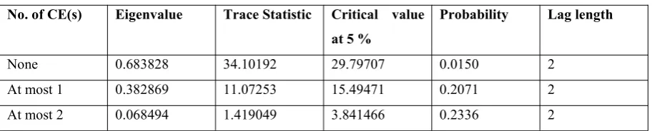
Table 3 shows the results of Johansen's Cointegration Trace test. Results of Johansen's Cointegration Trace test reveal that there is one Co-integrating equation at 5 percent significance level meaning that there is a long-run relationship between NOL, GDPG and RWAGE. Since in long run all the factors of production are variable the behavior of production when all the factors are varied remains the subject matter of economies of scale and economies of experience. It does so by allowing more output to be produced with the same level of employment, but with decreased cost of labour to firms. In the long run cost of a firm are not simply measured by the payment made towards the factors of production rather, it is measured by the costs and benefits relative to the output produced. Since in long run firms become specialized due to experience and large production, any increase in wages with a rise in labour productivity lowers the cost of labour thus firms will find it profitable to expand employment. With higher employment, potential GDP increases
Table-3: Trace Test No. of CE(s) Eigenvalue Trace Statistic Critical value
at 5 %
Probability Lag length
None 0.683828 34.10192 29.79707 0.0150 2 At most 1 0.382869 11.07253 15.49471 0.2071 2 At most 2 0.068494 1.419049 3.841466 0.2336 2
Note: Trace test indicates 1 co-integrating Eqn(s) at the 0.05 level
Vector Error Correction Model (VECM)
Having established the long-run relationship between the variables VECM has been performed to establish a link between the long-run equilibrium and the short-run dynamics. Since VECM allows for the long run behavior of the endogenous variable to converge to its long-run equilibrium while allowing for a wide range of short-run dynamics. Taking NOL as dependent variable and GDPG and RWAGE as independent variables the VECM model obtained is listed below:
D(NOL) = C(1)*( NOL(-1) - 2.65430404308e-06*GDPG(-1) + 3.04147505705e-05*RWAGE(-1) + 41.1684781412 ) + C(2)*D(NOL(-1)) + C(3)*D(NOL(-2)) + C(4)*D(GDPG(-1)) + C(5)*D(GDPG(-2)) + C(6)*D(RWAGE(-1)) + C(7)*D(RWAGE(-2)) + C(8)
D. Results of VECM
remove a large percentage of disequilibrium in each period meaning that speed of adjustment is very rapid.
Table-4: Results of VCEM
Error Correction Coefficient Std. Error t-statistics Prob.
Co-Integration model C(1) -2.091439 0.522877 -3.999868 0.0018
D(NOL(-1)) 0.171120 0.400956 1.986781 0.0577
D(NOL(-2)) 0.352710 0.414694 2.085053 0.0411
D(GDPG(-1)) -0.0000042 0.00000263 -2.597010 0.0136
D(GDPG(-2)) -0.00000579 0.00000241 -2.397559 0.0337
D(RWAGE(-1)) -0.0000345 0.0000196 2.763354 0.0103
D(RWAGE(-2)) -0.0000211 0.0000164 2.483047 0.0223
C8 32.35541 9.873260 3.277074 0.0066
6. CONCLUSIONS
Before proceeding to conclusions, we would like to mention that much care has been taken while designing and executing the study, however, still, some limitations remain. First, the data used in this study is an annual time series data. Second, the study focusses on the entire manufacturing sector without providing evidence for the sub- manufacturing sectors. Third, this study provides evidence from one country only. In this regard, future research can be conducted by taking into account the quarterly data across sub-manufacturing sectors and across a cross-section of countries. Such process will make the data a panel data and accordingly more robust estimates can be thought off.
To conclude, this study examined the linkage between labour, output and wages in Indian manufacturing sector. The results of Granger causality test indicated a bidirectional short run relationship between NOL and GDPG, RWAGE and GDPG and between RWAGE and NOL. Co-integration model affirms that long run relationship exists between labour, output and wages. Results of VECM show the speed of convergence to equilibrium is equal to 20.9 percent and the system is quite and the speed of adjustment is very rapid.
causing demand for workers to increase also in the short run. However, the substitution effect between the time spent on leisure and work implies that, as the wage rate increases leisure becomes relatively more expensive, meaning that, a labourer tends to increase the supply of labour by reducing the hours of leisure. While as long run relationship between NOL, GDPG and RWAGE is indicative of the fact that in long run firms become specialized due to experience and large production and any increase in wages with a rise in labour productivity lowers the cost of labour thus firms will find it profitable to expand employment. With higher employment, potential GDP increases. Therefore, there is mutual interdependence among the variables both in short and long term. Policies that promise to raise long-term growth should not be rejected on the grounds of that it might cut jobs in the short long-term.
The most appropriate level to analyze the relationship between labour, output and growth is the macro level (national level). Since wages are determined in the wider labour markets and the gains from the labour productivity is reflected in the reduced cost of output prices which ultimately boosts the demand, causing the GDP of the country to rise. Its effect seeps down into the micro level (sectorial level) and its benefits arise to everyone in the economy rather than workers only. Thus policy makers should be more concerned with the economic recovery and growth of country, should make changes in its macroeconomic policies that can help in making significant increase in labour employment, output and regulated wages. To increase employment in manufacturing industries, it is important to put focus on building more industries and improving the condition of present industries. The manufacturing sector of India has a significant potential to employ additional labour force. With every additional labour force employed this sector can increase the output thus contributing towards the GDP of the country.
REFERENCES
[1] Das, D. K., & Kalita, G. (2009). Do Labor Intensive Industries Generate Employment?: Evidence from firm level survey in India.
[2] Reserve Bank of India (2015-2016). Annual report. Available at
https://www.rbi.org.in/scripts/AnnualReportMainDisplay.aspx
[3] Altaf, N. (2016). Economic value added or earnings: What explains market value in Indian firms?.Future Business Journal,2(2), 152-166.
[4] Altaf, N., & Shah, F. A. (2015). Internationalization and firm performance of Indian firms: Does product diversity matter?.Pacific Science Review B: Humanities and Social Sciences,1(2), 76-84.
[5] Altaf, N., & Shah, F. A. (2016). Examining the Empirical Evidence for Environmental Kuznets Curve in Jammu and Kashmir.IIMS Journal of Management Science,7(3), 275-284.
[6] Planning Commission (2014-2015). Annual report. Available at
http://planningcommission.nic.in/plans/annualplan/ann_plan2014_15.pdf
[8] India Brand Equity Foundation (IBEF) (2010).Role of Manufacturing in Employment Generation in India. Available athttps://www.ibef.org/download/Role-of-Manufacturing-in-Employment-Generation-in-India.pdf
[9] Koutsogeorgopoulou, V. (1994). The impact of minimum wages on industrial wages and employment in Greece.International Journal of Manpower,15(2/3), 86-99.
[10] Cazes, S., & Verick, S. (Eds.). (2013). Perspectives on labour economics for development. International Labour Organization.
[11] ILO (2012). Wage-led growth: Concept, theories and Policies. Available at
http://www.ilo.org/wcmsp5/groups/public/---ed_protect/---protrav/---travail/documents/publication/wcms_192507.pdf
[12] McFarlane, A., Das, A., & Chowdhury, M. (2014). Non-linear dynamics of employment, output and real wages in Canada: Recent time series evidence.Journal of Economic Studies,41(4), 554-568.
[13] Islam, R., Kinyondo, A., & Nganga, J. (2015). Real wages and labour productivity in Tanzania: How do they link?.Journal of African Studies and Development,7(3), 81.
[14] Klein, N. (2012).Real wage, labor productivity, and employment trends in South Africa: A closer look(No. 12-92). International Monetary Fund
[15] Meager, N., & Speckesser, S. (2011). Wages, productivity and employment: A review of theory and international data.EEO Thematic Report, European Employment Observatory, 73.
[16] Mankiw, G. (2006). How are wages and productivity related?.Grege Mankiw’s Blog.
[17] Boltho, A., & Glyn, A. (1995). Can macroeconomic policies raise employment.Int'l Lab. Rev.,134, 451.
[18] Padalino, S., & Vivarelli, M. (1997). The employment intensity of economic growth in the G-7 countries.Int'l Lab. Rev.,136, 191.
[19] Sharpe, A., Arsenault, J. F., & Harrison, P. (2008).The relationship between labour productivity and real wage growth in Canada and OECD countries. Ottawa, Ontario: Centre for the Study of Living Standards.
[20] Serneels, P. (2005). Do wages reflect productivity?. Available at
https://ora.ox.ac.uk/objects/uuid:c5a4359f-b59f-4516-86f5-bfa790bfdc82/datastreams/ATTACHMENT01
[21] OECD (2007). “More Jobs but Less Productive? The Impact of Labour Market Policies on Productivity". Available athttp://www.oecd.org/employment/emp/40776638.pdf
[22] Gujarati, D. N. (2012).Basic econometrics. Tata McGraw-Hill Education.