2017
Predicting Adverse Outcomes in Chronic Kidney Disease Using
Predicting Adverse Outcomes in Chronic Kidney Disease Using
Machine Learning Methods: Data from the Modification of Diet in
Machine Learning Methods: Data from the Modification of Diet in
Renal Disease
Renal Disease
Zeid Khitan, Anna P. Shapiro, Preeya T. Shah, Juan R. Sanabria, Prasanna Santhanam, Komal Sodhi, Nader G. Abraham, and Joseph I. Shapiro
Follow this and additional works at: https://mds.marshall.edu/mjm
Part of the Nephrology Commons
Recommended Citation
Khitan, Zeid; Shapiro, Anna P.; Shah, Preeya T.; Sanabria, Juan R.; Santhanam, Prasanna; Sodhi, Komal; Abraham, Nader G.; and Shapiro, Joseph I. (2017) "Predicting Adverse Outcomes in Chronic Kidney Disease Using Machine Learning Methods: Data from the Modification of Diet in Renal Disease," Marshall Journal of Medicine: Vol. 3: Iss. 4, Article 10.
DOI: http://dx.doi.org/10.18590/mjm.2017.vol3.iss4.10
Available at: https://mds.marshall.edu/mjm/vol3/iss4/10
DOI: http://dx.doi.org/10.18590/mjm.2017.vol3.iss4.10
Author Footnote: The authors wish to acknowledge support from the National Institutes of Health (HL109015, HL071556 and HL105649 to J.I.S, HL34300 to N.G.A) as well as the
Brickstreet Foundation and the Huntington Foundation. The authors also wish to acknowledge access to the MDRD dataset furnished by the National Institutes of Health (NIDDK).
measurements in clinical trials. Modification of Diet in Renal Disease Study Group and the Diabetes Control and Complications Trial Research Group. Journal of the American Society of Nephrology : JASN. 1993;4(5):1159-71.
2. Levey AS, Gassman JJ, Hall PM, Walker WG. Assessing the progression of renal disease in clinical studies: effects of duration of follow-up and regression to the mean. Modification of Diet in Renal Disease (MDRD) Study Group. Journal of the American Society of Nephrology : JASN. 1991;1(9):1087-94.
3. Levey AS, Greene T, Sarnak MJ, Wang X, Beck GJ, Kusek JW, et al. Effect of dietary protein restriction on the progression of kidney disease: long-term follow-up of the Modification of Diet in Renal Disease
(MDRD) Study. Am J Kidney Dis. 2006;48(6):879-88. https://doi.org/10.1053/j.ajkd.2006.08.023
4. Levey AS, Adler S, Caggiula AW, England BK, Greene T, Hunsicker LG, et al. Effects of dietary protein restriction on the progression of advanced renal disease in the Modification of Diet in Renal Disease Study. Am J Kidney Dis. 1996;27(5):652-63. https://doi.org/10.1016/s0272-6386(96)90099-2
5. Levey AS, Berg RL, Gassman JJ, Hall PM, Walker WG. Creatinine filtration, secretion and excretion during progressive renal disease. Modification of Diet in Renal Disease (MDRD) Study Group. Kidney international Supplement. 1989;27:S73-80.
6. Levey AS, Greene T, Beck GJ, Caggiula AW, Kusek JW, Hunsicker LG, et al. Dietary protein restriction and the progression of chronic renal disease: what have all of the results of the MDRD study shown?
Modification of Diet in Renal Disease Study group. Journal of the American Society of Nephrology: JASN. 1999;10(11):2426-39.
7. CA G, MJ M, JI S, BL M. Predicting Medical Student Success on Licensure Exams. Med Sci Educ. 2015;25:447-53. https://doi.org/10.1007/s40670-015-0179-6
8. Tirelli T, Gamba M, Pessani D. Support vector machines to model presence/absence of Alburnus alburnus alborella (Teleostea, Cyprinidae) in North-Western Italy: comparison with other machine learning techniques. C R Biol. 2012;335(10-11):680-6. https://doi.org/10.1016/j.crvi.2012.09.001
9. Chen T, Cao Y, Zhang Y, Liu J, Bao Y, Wang C, et al. Random forest in clinical metabolomics for phenotypic discrimination and biomarker selection. Evid Based Complement Alternat Med. 2013;2013:298183. https://doi.org/10.1155/2013/298183
10. Khondoker MR, Bachmann TT, Mewissen M, Dickinson P, Dobrzelecki B, Campbell CJ, et al. Multifactorial analysis of class prediction error: estimating optimal number of biomarkers for various classification rules. J Bioinform Comput Biol. 2010;8(6):945-65. https://doi.org/10.1142/
s0219720010005063
11. Zhang Z. A gentle introduction to artificial neural networks. Ann Transl Med. 2016;4(19):370. https://doi.org/10.21037/atm.2016.06.20
12. Tsiliki G, Munteanu CR, Seoane JA, Fernandez-Lozano C, Sarimveis H, Willighagen EL. RRegrs: an R package for computer-aided model selection with multiple regression models. J Cheminform. 2015;7:46. https://doi.org/10.1186/s13321-015-0094-2
13. Liu R, Li X, Zhang W, Zhou HH. Comparison of Nine Statistical Model Based Warfarin
R and S+ to analyze and compare ROC curves. BMC Bioinformatics. 2011;12:77. https://doi.org/10.1186/ 1471-2105-12-77
15. Emir B, Johnson K, Kuhn M, Parsons B. Predictive Modeling of Response to Pregabalin for the Treatment of Neuropathic Pain Using 6-Week Observational Data: A Spectrum of Modern Analytics Applications. Clin Ther. 2017;39(1):98-106. https://doi.org/10.1016/j.clinthera.2016.11.015
16. Hengl T, Mendes de Jesus J, Heuvelink GB, Ruiperez Gonzalez M, Kilibarda M, Blagotic A, et al. SoilGrids250m: Global gridded soil information based on machine learning. PLoS One.
2017;12(2):e0169748. https://doi.org/10.1371/journal.pone.0169748
17. Gallo S, Hazell T, Vanstone CA, Agellon S, Jones G, L'Abbe M, et al. Vitamin D supplementation in breastfed infants from Montreal, Canada: 25-hydroxyvitamin D and bone health effects from a follow-up study at 3 years of age. Osteoporos Int. 2016. https://doi.org/10.1007/s00198-016-3549-z
Predicting adverse outcomes in chronic kidney disease using
machine learning methods: data from the modification of diet in renal
disease
Zeid Khitan MD1, Anna P. Shapiro MD2, Preeya T. Shah MS1, Juan Sanabria MD1, Prasanna Santhanam MD3,1, Komal Sodhi MD1, Nader G. Abraham PhD4,1, Joseph I. Shapiro MD1
Author Affiliation:
1. Marshall University Joan C. Edwards School of Medicine, Huntington, West Virginia 2. The Cleveland Clinic Foundation
3. John’s Hopkins University 4. New York Medical College
Corresponding Author:
Joseph I. Shapiro MD
Joan C. Edwards School of Medicine Huntington, West Virginia
Email: [email protected]
Acknowledgments:
The authors wish to acknowledge support from the National Institutes of Health (HL109015, HL071556 and HL105649 to J.I.S, HL34300 to N.G.A) as well as the Brickstreet Foundation and the Huntington Foundation. The authors also wish to acknowledge access to the MDRD dataset furnished by the National Institutes of Health (NIDDK). The MDRD study was
conducted by the MDRD Investigators and sup- ported by the National Institute of Diabetes and Digestive and Kidney Diseases (NIDDK). The data from the MDRD reported here were sup- plied by the NIDDK Central Repositories. This manuscript was not prepared in collaboration with the investigators of the MDRD study and does not necessarily reflect the opinions or views of the MDRD study, the NIDDK Central Repositories, or the NIDDK.
Statement of Ethics:
Abstract
Background: Understanding factors which predict progression of renal failure is of great interest to clinicians.
Objectives: We examined machine learning methods to predict the composite outcome of death, dialysis or doubling of serum creatinine using the modification of diet in renal disease (MDRD) data set.
Methods: We specifically evaluated a generalized linear model, a support vector machine, a decision tree, a feed-forward neural network and a random forest evaluated within the context of 10 fold validation using the CARET package available within the open source architecture R program.
Results: We found that using clinical parameters available at entry into the study, these computer learning methods trained on 70% of the MDRD population had prediction accuracies ranging from 66-77% on the remaining 30%. Although the support vector machine methodology appeared to have the highest accuracy, all models studied worked relatively well.
Conclusions: These results illustrate the utility of employing machine learning methods within R to address the prediction of long term clinical outcomes using initial clinical measurements.
Keywords
hypertension, blood pressure, chronic renal disease, correlation, machine learning, cardiovascular disease
Introduction
The modification of diet in renal disease study was a landmark clinical trial examining the effectiveness of blood pressure control and dietary protein restriction on renal disease progression.1 Although the maneuvers studied in the project were not very successful at attenuating renal disease progression, the most commonly used formula for estimating
glomerular filtration rate (eGFR) was developed from this study. We chose to use this data set to examine whether we could predict outcomes using different mathematical methodologies on this population.
Methods
A retrospective study was performed using data acquired in the “Modification of Diet in Renal Diseases” or MDRD study.2 Results from this study have been reported elsewhere.1-5 This data
measurement used was a composite variable consisting of death, dialysis or a doubling of the serum creatinine.6
All analysis was performed using the open source program R. We used a generalized linear (logistic regression) model as our default.7 In addition, we examined the utility of a support vector machine which involves the multi-dimensional sorting of data based on the development of a “hyperplane” which effectively separates the data.8 We also examined the performance of
decision trees with the RPART package and random forests with the randomForest package.9,10
The decision tree approach utilized three or more decisions. With the random forest technique, we found that the optimal number of trees was around nine. Different feed forward neural network architectures were explored using the nnet and neuralnet packages.11 We found optimal
performance with one hidden layer containing ten hidden neurons after this exploration. The CARET package was used for comparison of the mature models employing ten folds and three repeats.12 Other packages within R were used for different specific tasks (e.g., rminer to determine relative importance of variables, nnet for construction of the neural network, randomForest (RFor) for constructing random forests).11,13-17 Representative R routines for “cleaning the data” (e.g., centering and scaling, Appendix 2) splitting the data into training (70%) and testing (30%) sets, and comparing the different models with the categorical output (Appendix 3) are attached.
Results and Discussion
The MDRD study is famous for yielding clinical estimates of glomerular filtration rate, but it should be emphasized that it was developed to test whether dietary protein restriction would ameliorate the progression of renal failure. This study has been reviewed extensively elsewhere, but for the purpose of our interest, we had a group of patients with some degree of chronic kidney disease who developed a composite endpoint consisting of death, dialysis or a doubling of the baseline creatinine. Ergo, it was possible to fit the baseline data with different models.
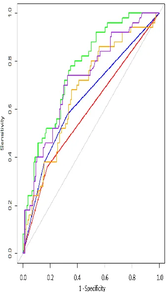
We found that each of the models studied had some success at prediction. It turns out that for each of the models, specificity was superior to sensitivity and accuracy ranged between 66 and 77%. When we examined the Receiver Operator Curves (ROC, Figure 1), it appears that the SVM and the RFor models performed somewhat better than the other models. When we
the relative size of the training and testing sets (varying from 50:50 to 85:15) also did not significantly affect our results (data not shown).
Figure 1: Receiver operator curves (ROC) showing sensitivity against 1-specificity for
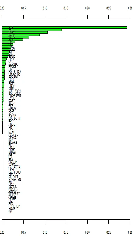
Figure 2: Relative importance of variables in the SVM model. Similar plots were produced and analyzed for all of the models studied. For all but the neural network model, the top three variables accounted for the vast majority of the model. The top three variables in importance for each model were as follows. GLM: SCr (serum [creatinine]), GFR (glomerular filtration rate) and Pro (proteinuria); SVM: SCr, Pro and Bicarb (serum [bicarbonate]); RPART: SCr, pack-years, and Pro; NNet: UPot (urinary [potassium], Packs (packs of cigarettes/day) and SCr, and RFor: SCr, GFR and Prot.
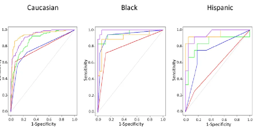
found that the predictive models performed similarly across the different racial subsets (Figure 3). It is important here to point out that the predictive value of these models was superior in these racial subsets to that achieved in the aforementioned randomly selected testing set, in part, because they were tested on some patients who were in the original training set. Therefore and due to these difficulties, ethnicity is an area that shows promise but will be explored later in another study with different dataset.
Figure 3: Receiver operator curves (ROC) showing sensitivity against 1-specificity for
generalized linear model (GLM) - red color, support vector machine (SVM) – green color, decision tree (RPART) – blue color, neural network (NNet) – orange color, random forest (RFor) – purple color, developed with the training set (70% of total) and applied to testing set consisting of all Caucasian, Black and Hispanic patients,
respectively. Note that some patients in these racial groups were used in both the training and testing sets. Although the linear model did not perform well in the Hispanic subset, other models especially the random forest, neural network and support vector machine models performed extremely well in all racial subsets.
References
1. Levey AS, Greene T, Schluchter MD, Cleary PA, Teschan PE, Lorenz RA, et al. Glomerular filtration rate measurements in clinical trials. Modification of Diet in Renal Disease Study Group and the Diabetes Control and Complications Trial Research Group. Journal of the American Society of Nephrology : JASN. 1993;4(5):1159-71.
2. Levey AS, Gassman JJ, Hall PM, Walker WG. Assessing the progression of renal disease in clinical studies: effects of duration of follow-up and regression to the mean. Modification of Diet in Renal Disease (MDRD) Study Group. Journal of the American Society of Nephrology : JASN. 1991;1(9):1087-94. 3. Levey AS, Greene T, Sarnak MJ, Wang X, Beck GJ, Kusek JW, et al. Effect of dietary protein restriction
on the progression of kidney disease: long-term follow-up of the Modification of Diet in Renal Disease (MDRD) Study. Am J Kidney Dis. 2006;48(6):879-88.
4. Levey AS, Adler S, Caggiula AW, England BK, Greene T, Hunsicker LG, et al. Effects of dietary protein restriction on the progression of advanced renal disease in the Modification of Diet in Renal Disease Study. Am J Kidney Dis. 1996;27(5):652-63.
5. Levey AS, Berg RL, Gassman JJ, Hall PM, Walker WG. Creatinine filtration, secretion and excretion during progressive renal disease. Modification of Diet in Renal Disease (MDRD) Study Group. Kidney international Supplement. 1989;27:S73-80.
6. Levey AS, Greene T, Beck GJ, Caggiula AW, Kusek JW, Hunsicker LG, et al. Dietary protein restriction and the progression of chronic renal disease: what have all of the results of the MDRD study shown? Modification of Diet in Renal Disease Study group. Journal of the American Society of Nephrology: JASN. 1999;10(11):2426-39.
7. CA G, MJ M, JI S, BL M. Predicting Medical Student Success on Licensure Exams. Med Sci Educ. 2015;25:447-53.
8. Tirelli T, Gamba M, Pessani D. Support vector machines to model presence/absence of Alburnus alburnus alborella (Teleostea, Cyprinidae) in North-Western Italy: comparison with other machine learning techniques. C R Biol. 2012;335(10-11):680-6.
9. Chen T, Cao Y, Zhang Y, Liu J, Bao Y, Wang C, et al. Random forest in clinical metabolomics for phenotypic discrimination and biomarker selection. Evid Based Complement Alternat Med. 2013;2013:298183.
10. Khondoker MR, Bachmann TT, Mewissen M, Dickinson P, Dobrzelecki B, Campbell CJ, et al. Multi-factorial analysis of class prediction error: estimating optimal number of biomarkers for various classification rules. J Bioinform Comput Biol. 2010;8(6):945-65.
11. Zhang Z. A gentle introduction to artificial neural networks. Ann Transl Med. 2016;4(19):370.
12. Tsiliki G, Munteanu CR, Seoane JA, Fernandez-Lozano C, Sarimveis H, Willighagen EL. RRegrs: an R package for computer-aided model selection with multiple regression models. J Cheminform. 2015;7:46. 13. Liu R, Li X, Zhang W, Zhou HH. Comparison of Nine Statistical Model Based Warfarin Pharmacogenetic
Dosing Algorithms Using the Racially Diverse International Warfarin Pharmacogenetic Consortium Cohort Database. PLoS One. 2015;10(8):e0135784.
14. Robin X, Turck N, Hainard A, Tiberti N, Lisacek F, Sanchez JC, et al. pROC: an open-source package for R and S+ to analyze and compare ROC curves. BMC Bioinformatics. 2011;12:77.
15. Emir B, Johnson K, Kuhn M, Parsons B. Predictive Modeling of Response to Pregabalin for the Treatment of Neuropathic Pain Using 6-Week Observational Data: A Spectrum of Modern Analytics Applications. Clin Ther. 2017;39(1):98-106.
16. Hengl T, Mendes de Jesus J, Heuvelink GB, Ruiperez Gonzalez M, Kilibarda M, Blagotic A, et al. SoilGrids250m: Global gridded soil information based on machine learning. PLoS One.
2017;12(2):e0169748.
Table 1: Confusion Matrices with Different Models
Model Yes No Specificity Sensitivity Accuracy
Reference 50 134
GLM 18/50 100/134 82% 36% 64%
SVM 23/50 119/134 89% 46% 77%
RPart 21/50 108/134 81% 42% 70%
NNet 19/50 102/134 76% 38% 66%
RForest 20/50 114/134 85% 40% 73%
Appendix 1: Var Name "STDWT" "CURHT" "WEIGHT" "BMI" "GFR" "MAP1" "UCRE" "UUN" "UPHO" "UVOL" "UPOT" "SUN" "SCR" "TCHOL" "TRAN" "ALB" "HBA1C" "PHOS" "TRIG" "LDL" "HDL" "POT" "BICARB" "CAL" "MG" "HB" "HCT" "DPRO" "DCALS" "DPHOS" "IRON" "WBC" "MAP" "UNEPI" "STUDY" "DIET" "PRO" "SYS" "DIA" Var Description Ideal Weight Height Weight
Body Mass Index
Glomerular Filtration Rate Mean Arterial Pressure 1 Urinary [Creatinine] Urinary [Urea Nitrogen] Urinary [Phosphate] Urine Volume Urine [Protein] Serum Urea Nitrogen Serum Creatinine Total Cholesterol Transferrin Albumin HBA1C Serum Phosphate Serum Triglycerides Low Density Lipoprotein High Density Lipoprotein Serum Potassium Serum Bicarbonate Serum Calcium Serum Magnesium Hemoglobin Hematocrit Dietary Protein Dietary Calcium Dietary Phosphate Serum Iron
White Blood Cells Mean Arterial Pressure during Study
UNEPI Study Group Diet Study Protein Study
Systolic Blood Pressure Diastolic Blood Pressure
Var Name "UNADJGFR" "BSA" "HT" "RACE" "EDUC" "OCCUP" "HOME" "EMPL" "RELDIET" "MARSTAT" "ALONE" "DIAB" "CAD" "PEPULC" "CANCER" "CVD" "PVD" "HYPERTEN" "HYPERLIP" "SURGERY" "PACKS" "YEARS" "Pyr" "SODIUM" "CHLORIDE" "URIC" "BILI" "LDH" "SGOT" "GLUC" "POT_FOOD" "POT_BOTH" "SOD_FOOD" "SOD_BOTH" "CAL_FOOD" "CAL_BOTH" "B0AGE" Var Description
GFR not adjusted Body Surface Area Height during study Race
Education level Occupation code Stay at Home Employment Diet Group Marital Status Live Alone Diabetic
Coronary Artery Disease Peptic Ulcer
Cancer Stroke
Peripheral Vascular Disease Hypertension
Hyperlipidemia Prior Surgery
Smoking packs per day Years smoking
Product of prior two Serum Sodium Serum Chloride Serum Uric Acid Serum Bili Serum LDH
Alanine Transaminase Serum Glucose
Potassium from food Total Potassium Sodium from food Total Sodium Calcium from food Total Calcium
Appendix 2: Cleaning Data
#call in data set, remove patient index variable xx=x[2:86]
# only complete cases xx=xx[complete.cases(xx),] dim(xx)
#create yes no variable for outcome k=NULL
for(i in 1:dim(xx)[1]){ if(xx$EV_ALL[i]>0){ k[i]="yes"
}else{ k[i]="no" }
}
#create set for analysis z=xx[,2:77]
z=cbind(z,k)
colnames(z)[77]="output1" #scale and center data
Appendix 3: ROC curve and model analysis
#load libraries library(ROCR) library(pROC) library(rpart) library(caret) library(nnet) library(C50) library(ggplot2) library(lattice)
library(randomForest) library(rminer)
# produce copy in a text file sink('output1_2.txt', split=TRUE)
# separate the “cleaned” dataset z randomly into training and testing sets set.seed(2)
ind = sample(2, nrow(z), replace = TRUE, prob = c(0.75, 0.25)) trainset = z[ind == 1,]
testset = z[ind == 2,]
# train the different models within CARET on the training set
control = trainControl(method = "repeatedcv", number = 10, repeats = 3, classProbs = TRUE, summaryFunction = twoClassSummary)
glm.model = train(output1 ~ ., data = trainset, method = "glm", metric = "ROC", trControl = control)
svm.model = train(output1 ~ ., data = trainset, method = "svmRadial",metric = "ROC", trControl = control)
rpart.model = train(output1 ~ ., data = trainset, method = "rpart", metric = "ROC", trControl = control)
tunGrid=expand.grid(size=c(5),decay=c(0.1))
nnet.model = train(output1 ~ ., data=trainset, method = "nnet", metric="ROC", trControl=control, tuneGrid=tunGrid)
rfor.model = train(output1 ~ ., data=trainset, method = "rf", metric="ROC", trControl=control)
# establish predictions from these models on the testing set
rpart.probs = predict(rpart.model, testset[,! names(testset) %in% c("output1")], type = "prob") nnet.probs=predict(nnet.model, testset[,! names(testset) %in% c("output1")], type = "prob") rfor.probs=predict(rfor.model, testset[,! names(testset) %in% c("output1")], type = "prob")
#create receiver operator curves windows()
glm.ROC = roc(response = testset[, c("output1")], predictor = glm.probs$yes, levels = levels(testset[, c("output1")]))
plot(glm.ROC,add=F, col =" red")
svm.ROC = roc(response = testset[, c("output1")], predictor = svm.probs$yes, levels = levels(testset[, c("output1")]))
plot(svm.ROC, add = TRUE, col ="green")
rpart.ROC = roc(response = testset[, c("output1")], predictor = rpart.probs$yes, levels = levels(testset[, c("output1")]))
plot(rpart.ROC, add = TRUE, col ="blue")
nnet.ROC=roc(response = testset[, c("output1")], predictor = nnet.probs$yes, levels = levels(testset[, c("output1")]))
plot(nnet.ROC, add = TRUE, col ="orange")
rfor.ROC=roc(response = testset[, c("output1")], predictor = rfor.probs$yes, levels = levels(testset[, c("output1")]))
plot(rfor.ROC, add = TRUE, col ="purple")
#produce confusion matrices
glm.pred=predict(glm.model,testset[,!names(testset)%in% c("output1")]) table(glm.pred,testset[,c("output1")])
confusionMatrix(glm.pred,testset[,c("output1")])
svm.pred=predict(svm.model,testset[,!names(testset)%in% c("output1")]) table(svm.pred,testset[,c("output1")])
confusionMatrix(svm.pred,testset[,c("output1")])
rpart.pred=predict(rpart.model,testset[,!names(testset)%in% c("output1")]) table(rpart.pred,testset[,c("output1")])
confusionMatrix(rpart.pred,testset[,c("output1")])
nnet.pred=predict(nnet.model,testset[,!names(testset)%in% c("output1")]) table(nnet.pred,testset[,c("output1")])
confusionMatrix(nnet.pred,testset[,c("output1")])
table(rfor.pred,testset[,c("output1")])
confusionMatrix(rfor.pred,testset[,c("output1")])
#determine variable importance in different models
model_rpart=fit(output1~., trainset, model="dt")
VI_rpart=Importance(model_rpart,trainset,method="sensv")
L_rpart=list(runs=1,sen=t(VI_rpart$imp), sresponses=VI_rpart$sresponses) windows()
mgraph(L_rpart,graph="IMP",leg=names(trainset),cex=0.6,col="blue")
model_rfor=fit(output1~., trainset, model="randomForest") VI_rfor=Importance(model_rfor,trainset,method="sensv")
L_rfor=list(runs=1,sen=t(VI_rfor$imp), sresponses=VI_rfor$sresponses) windows()
mgraph(L_rfor,graph="IMP",leg=names(trainset),cex=0.6, col="purple")
model_glm=fit(output1~., trainset, model="cv.glmnet") VI_glm=Importance(model_glm,trainset,method="sensv")
L_glm=list(runs=1,sen=t(VI_glm$imp), sresponses=VI_glm$sresponses) windows()
mgraph(L_rfor,graph="IMP",leg=names(trainset),cex=0.6,col="red")
model_nn=fit(output1~., trainset, model="mlpe") VI_nn=Importance(model_nn,trainset,method="sensv")
L_nn=list(runs=1,sen=t(VI_nn$imp), sresponses=VI_nn$sresponses) windows()
mgraph(L_nn,graph="IMP",leg=names(trainset),cex=0.6,col="orange")
model_svm=fit(output1~., trainset, model="svm")
VI_svm=Importance(model_svm,trainset,method="sensv")
L_svm=list(runs=1,sen=t(VI_svm$imp), sresponses=VI_svm$sresponses) windows()