S O F T W A R E
Open Access
An R package for analyzing and modeling
ranking data
Paul H Lee
1,2*and Philip LH Yu
2Abstract
Background:In medical informatics, psychology, market research and many other fields, researchers often need to analyze and model ranking data. However, there is no statistical software that provides tools for the comprehensive analysis of ranking data. Here, we present pmr, an R package for analyzing and modeling ranking data with a bundle of tools. The pmr package enables descriptive statistics (mean rank, pairwise frequencies, and marginal matrix), Analytic Hierarchy Process models (with Saaty’s and Koczkodaj’s inconsistencies), probability models (Luce model, distance-based model, and rank-ordered logit model), and the visualization of ranking data with multidimensional preference analysis.
Results:Examples of the use of package pmr are given using a real ranking dataset from medical informatics, in which 566 Hong Kong physicians ranked the top five incentives (1: competitive pressures; 2: increased savings; 3: government regulation; 4: improved efficiency; 5: improved quality care; 6: patient demand; 7: financial incentives) to the computerization of clinical practice. The mean rank showed that item 4 is the most preferred item and item 3 is the least preferred item, and significance difference was found between physicians’preferences with respect to their monthly income. A multidimensional preference analysis identified two dimensions that explain 42% of the total variance. The first can be interpreted as the overall preference of the seven items (labeled as“internal/ external”), and the second dimension can be interpreted as their overall variance of (labeled as“push/pull factors”). Various statistical models were fitted, and the best were found to be weighted distance-based models with Spearman’s footrule distance.
Conclusions:In this paper, we presented the R package pmr, the first package for analyzing and modeling ranking data. The package provides insight to users through descriptive statistics of ranking data. Users can also visualize ranking data by applying a thought multidimensional preference analysis. Various probability models for ranking data are also included, allowing users to choose that which is most suitable to their specific situations.
Keywords:Distance-based model, Luce model, Multidimensional preference analysis, Visualization, Weighted distance
Background
Ranking data arises when a number of items are to be ranked. By the nature of the ranking data, they can be di-vided into two types. The first type is characterized by a small number of items to be ranked, and they frequently represent the preference of these items among a group of judges (individuals). These items can be candidates in an
election [1], one’s place of living [2], choice of occupations [3,4], medical treatment [5], and so on. In analyzing these data, the focus is on the judges’perception and preference of some specific (or all) items. In recent years, this type of ranking data have also becoming more popular in the medical literature, particularly in health economics [6-10] and medical informatics [11].
The second type of ranking data is characterized by a large number of items, and they frequently represent the ordering of these items in which researchers would like to determine or predict which items were ranked at the top positions. Examples of such ranking data include search engine results [12], integration of microRNA and
* Correspondence:[email protected] 1
School of Public Health/Department of Community Medicine, The University of Hong Kong, Room 624-627, Core F, Cyberport 3, 100 Cyberport Road, Hong Kong, Hong Kong
2Department of Statistics and Actuarial Science, The University of Hong
Kong, Hong Kong, Hong Kong
mRNA [13], and consumer behavior in e-commerce ap-plications [14]. Due to the large number of items, these ranking datasets often contain missing or tie rankings, which are impossible to analyze without computers. With the decreasing cost of powerful computers, more researchers have paid attention to this type of ranking data, especially those in machine learning and know-ledge discovery.
Analyzing and modeling ranking data is an efficient way to understand people’s perceptions and preferences for different items. Over the years, besides statistical tests for hypothesis testing [15], various models have been developed for ranking data, including the Luce model [16], distance-based model [1], ϕ-component model [17] and weighted distance-based model [18,19].
The maximum likelihood estimator (MLE) of the aforementioned models does not have a closed form, yet the MLE can be obtained using iterative algorithms. However, at present, only summary statistics and a visualization of ranking data are available (partially and indirectly) in some statistical software (for example, pro-cedure MDPREF in SAS), not to mention hypothesis testing and probability models for ranking data. The lack of software and tools for analyzing ranking data is not a problem for statisticians who are used to writing pro-grams for their own means. However many scientists are not familiar with programming. We believe that a single package for the analysis of ranking data could offer users a more complete analysis, allowing them to use a single program instead of shifting their ranking datasets from one application to another.
R [20], an open-source program for statistical analysis, is gaining in popularity because of its high flexibility.
Indeed, users are free to write/use packages for specific purposes. Although many packages are highly relevant to medicine [21,22], there are only a limited number of packages for analyzing and modeling ranking data. There are some basic tools for ranking data, for example the
Kendallpackage and thepspearmanpackage for the com-putation of Kendall and Spearman rank correlation. None-theless, to the best of the authors’ knowledge, the only statistical model currently available in R is the RMallow
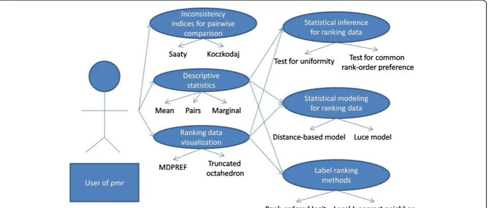
package (http://cran.r-project.org/web/packages/RMallow) for fitting a mixture of Mallows’ models [23]. Here, we present pmr (probability models for ranking data), an R package for analyzing and modeling ranking data with a bundle of statistical tools. A review of statistical analysis for ranking data is given, prior to demonstrating the im-plementation ofpmr. The current version ofpmrand the user manual can be found in Additional files 1 and 2 respectively. In addition, four ranking models are reviewed, namely the Luce model, distance-based model, ϕ-component model, and weighted distance-based model. For more details, readers can refer to [15,24,25]. The use cases diagram of thepmrpackage is shown in Figure 1.
Implementation
In this section, we give a review of statistical analyses for ranking data. For a better description of ranking data, some notations must be defined. For a set ofkitems, labelled 1, …,k, a rankingπis a mapping function from 1,…,kto 1,…,
k, where π(i) is the rank given to item i. For example, π(2) = 3 means that item 2 has a rank of 3. The inverse of the ranking function (sometimes referred to as ordering) π-1
(i) is defined as the item that has ranki. For example, π-1
(5) = 6 means that the item with rank 5 is item 6.
Descriptive statistics for ranking data
Descriptive statistics give an overall picture of the rank-ing dataset. Not only do descriptive statistics provide a summary of the ranking dataset, but they also lead us in an appropriate direction to analyze the dataset. There-fore, it is suggested that researchers consider descriptive statistics prior to any sophisticated analysis of ranking data.
We begin with a single measure of the popularity of an item. It is natural to use the mean rank attributed to an item to represent the central tendency of the ranks. Mean rank mis defined as the k-dimensional vector in which thejth entry equals
mj¼ Xk!
i¼1
Niπið Þj ;
where πi, i= 1, 2, …, k! represents all possible rankings
of thekitems,Niis the observed frequency of rankingi, andπi(j) is the rank given to itemjin rankingi.
Apart from the mean ranks, the pairwise frequencies, that is, the frequency with which itemiis ranked higher than itemjfor every possibleCk2item pairs (i,j), are also often used. These pairwise frequencies can be summa-rized in a k×kmatrix called a pair matrix (P) in which the (s,t)thentry equals
Pst¼ Xk!
i¼1
NiI½πið Þs >πið Þt ;
whereI[·] is the indicator function. Note thatPst/N rep-resents the empirical probability that item s is ranked higher than itemt. In addition to mean ranks and pair-wise frequencies, one can look more deeply into a rank-ing dataset by studying the so-called “marginal” distribution of the items. A marginal matrix, specifically for this use, is the k×k matrix M in which the (s,t)th entry equals
Mst ¼ Xk!
i¼1
NiI½πið Þ ¼s t:
Note thatMst is the frequency of items being ranked
tth. It is called a marginal matrix because “the ith row gives the observed marginal distribution of the ranks assigned to itemi, and thejthcolumn gives the marginal distribution of objects given the rankj.”([15], page 18).
Inconsistency indices for pairwise comparisons
According to the Analytic Hierarchy Process [26], a group of judges combine the rankings from different cri-teria to form a final ranking. The Analytic Hierachy Process has been used to determine the weights of these criteria. First, a pairwise comparison matrixA, in which
the (s,t)thentryast equals the number of times criterion
s is preferred over criteriont, is computed. The weights are then found as the eigenvalues of the matrix A. The reliability of these weights depends on the consistency of the ranking process, which is defined asastatu=asufors,
t, u= (1,…, k). Therefore, evaluating the consistency of the ranking data using A is a crucial task in analyzing ranking data and hence a number of measures have been developed for this purpose. One popular measure is Saaty’s index, which is given by
λmax−k
k−1
RIk ;
whereλmaxis the largest eigenvalue ofA, andRIk is the
average value ofλmax−k
k−1 for ak×krandom matrix. Another
popular measure is Koczkodaj’s index, which equals max min 1 −acb;1−acbfor each triad (a,b,c) inA}.
Other consistency indices exist besides these two [27].
Visualizing ranking data: multidimensional preference analysis
Because ranking data often have a high dimension, visualization is a good first step towards their analysis. Multidimensional preference analysis [28] is a dimension reduction technique that aims to display ranking data in a low-dimensional (preferably 2D or 3D) space. It is ap-plicable to ranking data with five or more items where the dataset cannot be displayed in a 2D/3D plot. Let X
be an N×k matrix of ranking data such that xij repre-sents the rank of itemjassigned by judgei, centered by the overall mean rank, i.e., (k+ 1)/2. Suppose the singu-lar value decomposition of X is X=UDV’. A 2D repre-sentation of the multidimensional preference analysis denotes the items and judges by the first two columns offfiffiffiffiffiffiffiffiffiffi
N−1 p
U and DVffiffiffiffiffiffiffi′
N−1
p , respectively. Items are usually plotted
as points, whereas judges are plotted as vectors from the origin. To give a better graphical display, the length of the ranking vectors can be scaled to fit the position of the items. It is not difficult to see that the perpendicular projection of all k item points onto a judge vector will closely approximate the ranking of the k items by that judge if the 2D solution fits the data well. Otherwise, we may look for a higher-dimension solution.
Statistical inferences for ranking data
When we say that a ranking dataset is uniform, we mean that all possible rankings have the same probabil-ity of being observed. Hence, under uniformprobabil-ity, the expected frequencies of every ranking should be N/k!, and the standard χ2test can be applied to test the uni-formity. However, when k! is too large compare with N, this is not always applicable, because we may encounter rankings with fewer than five observation. In such a case, mean rank, pairs, or marginals can be used to test the uniformity instead of ranking proportions [15]. Note that under uniformity, the expected values of mean rank, pairs, and marginals are (k+ 1)/2, 0.5N, and N/k
respectively.
Under uniformity, the test statistic when using mean rank, pairs, and marginals are ([15], page 58, Table 3.1)
12N k kð þ1Þ
Xk
j¼1
mj−
kþ1 2
2
;
12N X
k
s>t
Pst−0:5 !2
−
Xk
s>t
mj−
kþ1 2
!2
kþ1
2 6 6 6 6 4
3 7 7 7 7 5;and
N Kð þ1ÞX k
s>t
Mst− 1
k
2
;
and they follow a χ2 distribution with k-1, Ck
2, and (k
-1)2 degrees of freedom, respectively.
Theχ2test could be used to test for any difference be-tween two ranking datasets. Before doing so, we align the matrix (in the case of pairs and marginals) into a
q× 1 vector, for both datasets. We can now use the standard χ2 test. For comparison between three or more ranking datasets, MANOVA-like tests can be used [15].
Statistical models for ranking data: the Luce model After conducting a descriptive analysis for ranking data, we may have some understanding about the empirical distribution of the rank-order preferences of different items and their popularity. To further understand the data and make inferences about its structure, an effi-cient method is to establish some statistical models for ranking data. Over the years, various statistical models for ranking data have been developed. In this subsection, we review a commonly used approach, the Luce model.
Supposenjudges are asked to rank kitems. Luce [29] proposed a ranking process where independent utilities
V= (V1, V2,..,Vk)≥0 are assigned to item 1,2, …,k. The probability of observing rankingπnis
PðπjVÞ ¼Y
k−1
j¼1
Vπ−1
nð Þj
Xk
i¼j
Vπ−1
nð Þi
;
and the resulting models is referred to as the Luce models [16]. The Luce models can be interpreted as a vase model [15]: imagine there are infinitely many balls inside a vase, and each ball is labeled j., j= 1, 2, …, k. The proportion of balls labeled withj is proportional to
Vj. Then, the Luce models correspond to the ranking process whereby the first ball drawn is labeledπ-1(1), the second ball drawn is labeledπ-1(2) (with all balls labeled π-1
(1) removed from the vase), and the process con-tinues until all balls in the vase have the same label.
The loglikelihood function is globally concave, and hence a global maximum exists. The MLE of the param-eters can thus be obtained using standard methods, e.g., the Newton–Raphson algorithm. Besides MLE, Bayesian method can also be used for parameter estimation, using expectation propagation [30], generalized repeated inser-tion model [31], and random atomic measures [32].
The Luce model can be extended to incorporate covar-iates. We can include Mcovaraites of judgen,xmn, m= 1, 2,…,M, into the utilities, that is,
Vnj¼βj0þ
XM
m¼1
βjmxnm;
where βjm, m= 0, 1, 2, …, M are parameters specific to
itemj. This extension of the Luce model is known as the rank-ordered logit (ROL) model [33-35].
Statistical models for ranking data: distance-based model In what follows, we will introduce the distance-based model for ranking data. Before doing so, we need to have a clear definition of the“distance”between two rankings. A distance function is useful in measuring the discrep-ancy between two rankings. The usual properties of a distance function between two rankingsπandσare:
dðπ; πÞ ¼0;
dðπ; σÞ>0 if π≠σ;
dðπ; σÞ ¼dðσ; πÞ:
invariant, i.e.,d(π,σ) =d(π○γ,σ○γ), whereπ○γ(i) =π(γ(i)). This requirement ensures that the relabeling of items has no effect on the distance.
Some popular right-invariant distances are Spearman’s rho [36], given by
Rðπ;σÞ ¼ X
k
i¼1
πð Þi−σð Þi
½ 2
!0:5
;
Spearman’s rho square, given by
R2ðπ;σÞ ¼X
k
i¼1
πð Þi −σð Þi
½ 2;
Spearman’s footrule, given by
Fðπ;σÞ ¼X
k
i¼1
πð Þi −σð Þi
j j;
and Kendall’s tau, given by
Tðπ;σÞ ¼ ∑
i<jIf½πð Þi −πð Þj½σð Þi −σð Þj<0g;
where I() is the indicator function. There are other dis-tances applicable to ranking data, and readers can refer to [24] for details.
It is reasonable to assume that there is a modal rank-ing π0, and we expect most of the judges to have
rank-ings close toπ0. According to this framework, Diaconis
[1] developed a class of distance-based models,
Pð jπλ;π0Þ ¼
e−λdðπ;π0Þ Cð Þλ ;
whereλ> 0 is the dispersion parameter,C(λ) is the pro-portionality constant, and d(π, π0) is an arbitrary right
invariant distance. When we use Kendall’s tau as the dis-tance function, the model is called Mallows’ ϕ-model [37]. In distance-based models, rankings nearer to the modal ranking π0 have a higher probability of
occur-rence and this is controlled by λ. The distribution of rankings will be more concentrated around π0 for a
smaller value ofλ.
A closed form for the proportionality constant C(λ) only exists for some distances. In principle, it can be solved numerically by summing e−λdðπ; π0Þ over all
possible π. The computational time increases exponen-tially with the number of items [17].
Statistical models for ranking data:ϕ-component model Fligner and Verducci [17] extended the distance-based models by decomposing the distance metricd(π, σ) into k-1 distance metrics,
dðπ;σÞ ¼X
k−1
i¼1
diðπ;σÞ; ð1Þ
where each di(π, σ)is independent. Both Kendall’s tau
and Cayley’s distance [38] can be decomposed in this form, and Fligner and Verducci [17] developed two new classes of ranking models for these, calledϕ-component models and cyclic structure models, respectively.
Fligner and Verducci [17] showed that Kendall’s tau satisfies [1]:
Tðπ;π0Þ ¼
Xk−1
π0ð Þ¼i 1 Vπ0ð Þi;
where
Vπ0ð Þi ¼ Xk
π0ð Þ¼j π0ð Þþi 1
If½πð Þi−πð Þj>0g:
Here,V1represents the number of adjacent transposi-tions required to place the best item in π0 in the first
position.V2is the number of adjacent transpositions re-quired to place the second best item inπ0in the second
position, and so on. Therefore, the ranking can be de-scribed as k-1 stages,V1 to Vk-1, where Vi=m can be interpreted asmmistakes made in stagei.
By applying a dispersion parameter λito stage Vi, the
Mallows’ϕ-model is extended to:
Pð jπΛ;π0Þ ¼
e
− X k−1
π0ð Þ¼i 1
λπ0ð ÞiVπ0ð Þi
Cð ÞΛ ;
whereΛ= {λi,i= 1,…,k= 1} andC(Λ) is the
proportion-ality constant, which equals
Yk−1
π0ð Þ¼i 1
1−e−ðk−π0ð Þþi 1Þλπ0ð Þi
1−e−λπ0ð Þi :
ϕ-component models in other papers [24]. Mallows’ ϕ -models are special cases of ϕ-component models whenλ1=…=λk-1.
Statistical models for ranking data: weighted distance-based model
Lee and Yu [18,19] proposed an extension of the distance-based model by replacing the (equal-weighted) distance with a new weighted distance measure, so that different weights can be assigned to different ranks.
Motivated by the weighted Kendall’s tau correlation coefficient [39], Lee and Yu [18,19] defined the weighted Kendall’s tau distance by
Twðπ;σÞ ¼ ∑
i<jwπ0ð Þiwπ0ð ÞjIf½πð Þi −πð Þj ½σð Þi−σð Þj<0g:
It is important to note that this weighted distance sat-isfies all the usual distance properties, in particular the symmetry property, i.e.,Tw(π,σ) =Tw(σ,π).
Other distance measures can be generalized to a weighted distance in a similar manner to this generalization of Kendall’s tau distance. For examplethe weighted Spearman’s rho is
Rwðπ;σÞ ¼ Xk
i¼1
wπ0ð Þi½πð Þi −σð Þi
2
!0:5
;
The weighted Spearman’s rho square is
R2wðπ;σÞ ¼X
k
i¼1
wπ0ð Þi½πð Þi −σð Þi
2;
and the weighted Spearman’s footrule is
Fwðπ;σÞ ¼ Xk
i¼1
wπ0ð Þijπð Þi−σð Þi j:
Apart from the weighted Kendall’s tau [39] and weighted Spearman’s rho square [40], many other weighted rank correlations have been proposed [41].
Applying a weighted distance measure dw to the
distance-based model, the probability of observing a rankingπbecomes
Pð jπw;π0Þ ¼
e−dwðπ;π0Þ C wð Þ :
Generally speaking, if wi is large, few people will tend to disagree that the item ranked i in π0 should not be
ranked i. This is because such disagreement will greatly increase the distance and hence the probability of ob-serving it will become very small. If wi is close to zero, people have little or no preference on how the item ranked i in π0 is ranked, because a change in its rank
will not affect the distance at all. The extension of weighted distance-based ranking models can retain the nature of distance, and at the same time maintain a greater flexibility. Readers are referred to [19] for the de-tails of these properties.
Label ranking method usingk-nearest neighbor algorithm
Label ranking is defined as the problem of classifying a judge’s ranking over a set of items given the covariate of this judge and a training dataset. ROL can be used for this, as it produces utility scores that can generate rank-ings for the judges. However, when the number of items and covariate are large, ROL may not be feasible due to its long computation time. Recently, a local k-nearest neighbor method has been developed for label rank-ing [42]. If we want to predict the rankrank-ing of judge i, we can first select the k-nearest neighbor (by Euclid-ean distance) of i. Second, a statistical model (the Luce model in [42]) is fitted to these k neighbors and the parameters will be used to predict the ranking of judge i.
Results and discussion
rankings and their corresponding frequencies. To transform the individual ranking data to an aggre-gated format, the rankagg function can be used (q4agg < - rankagg(q4)).
All analyses of ranking data start from descriptive sta-tistics. Using the R code destat(q4agg), the destat func-tion produces the mean rank vector, the pairs matrix, and the marginal:
From the descriptive statistics, we can deduce that item 4, improved efficiency, is the most preferred item, and item 3, government regulation, is the least preferred item.
Statistical inferences about ranking data can be performed using the destatfunction. For instance, if we want to test whether the ranking over seven items is uni-form using mean rank, the following R code can be input:
and would give the output:
The χ2 test statistic equals 524.8747 and the corre-sponding p-value equals 1.82345 × 10-110. Thus, the ranking was not uniformly distributed.
This example illustrates how to test the uniformity of a ranking dataset using the destatfunction, and we will now explain how to compare two ranking datasets using the same function. For example, we may wish to test the hypothesis that physicians with monthly incomes above and below HK$100,000 (rankings stored in q4agg. highincome and q4agg.lowincome respectively) have dif-ferent preferences towards computerization incentives. According to the marginal matrix using the χ2 test, the following codes:
give the output:
Theχ2test statistic equals 66.415 and the correspond-ing p-value equals 0.04. Thus, we have found a signifi-cant difference between physicians’ preferences with respect to their monthly income.
Multidimensional preference analysis [28] can help us understand more about the physicians’ ranking process and their preferences over the seven items by decomposing the rankings into a few dimensions. This can be performed using the mdpref function (R de1 <- destat(q4agg); mean <- rep(4,7);
chi <- 12*567*sum((de1$mean.rank - mean)^2 )/7/8;
chi; dchisq(chi,6)
> chi
[1] 524.8747
> dchisq(,6)
[1] 1.82345e-110
[,1] [,2] [,3] [,4] [,5] [,6] [,7]
[1,] 0 330 433 189 240 353 310
[2,] 236 0 421 182 214 324 281
[3,] 133 145 0 123 141 280 220
[4,] 377 384 443 0 386 441 422
[5,] 326 352 425 180 0 422 385
[6,] 213 242 286 125 144 0 287
[7,] 256 285 346 144 181 279 0
$mar
[,1] [,2] [,3] [,4] [,5] [,6] [,7]
[1,] 73 93 89 88 109 114 0
[2,] 71 55 91 88 82 165 14
[3,] 29 29 48 62 94 157 147
[4,] 213 116 70 72 36 27 32
[5,] 81 163 105 72 57 39 49
[6,] 41 51 71 92 86 64 161
[7,] 58 59 92 92 102 0 163 Descriptive statistics of ranking data:
$mean.rank: mean ranks; $pair: pairs; $mar: marginals
$mean.rank
[1] 3.722615 4.070671 5.159011 2.666078 3.307420 4.708481
4.365724
$pair
de.highincome <- destat(q4agg.highincome)
de.lowincome <- destat(q4agg.lowincome)
chisq.test(cbind(as.vector(de.highincome$mar),as.vector(de.low
income$mar)))
> Pearson's Chi-squared test
> data: cbind(de.highincome$mar,de.lowincome$mar)
code: mdpref(q4agg,rank.vector = T)). The output is as follows:
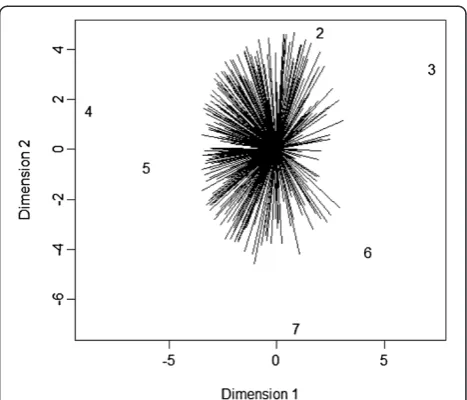
and the 2D plot is given in Figure 2.
The coordinates of the items and rankings, and the proportion of variance explained by the first two dimen-sions are stored in the values $item, $rankingand
$ex-plain respectively. The final two columns of the
$rankingmatrix are the coordinates of the first two col-umns of DVffiffiffiffiffiffiffi′
N−1
p .
Figure 2 shows the multidimensional preference graph. The 2D plot explains around 42 % of the total variance. The first dimension can be interpreted as the overall preference of the seven items (labeled as“ internal/exter-nal”). The leftmost item (item 4) and rightmost item (item 3) are the most and the least preferred items, re-spectively. The second dimension can be interpreted as the overall variance of the seven items (labeled as“push/ pull factors”). The bottommost item (item 7) has the lar-gest variance and the topmost item (item 2) has the sec-ond largest variance among the seven items.
Descriptive statistics and plots provide an insight to the data, but modeling will be more useful if we wish to have a deeper understanding. The Luce model (pl), distance-based model (dbm), ϕ-component model (phicom) and weighted distance-based model (wdbm)
can be fitted using the pmr, which requires the stats4
package. We will demonstrate the model fitting proced-ure. Spearman’s footrule distance usually gives the best fit [18,19] and hence it will be used in our demonstra-tion of distance-based models.
The parameter estimates of the Luce model can be obtained using the R code q4.pr <- pl(q4agg); q4.pr@coef, and the output is as follows:
The warning messages are a result of some of the pre-dicted probabilities being close to zero. The parameter estimates of the distance-based model can be obtained using the R code q4.dbm < - dbm(q4agg); q4.dbm@coef, and the distance type can be specified using the argu-ment dtype (default: Kendall’s tau; rho: Spearman’s rho;
rho2: Spearman’s rho square;foot: Spearman’s footrule). The loglikelihood is a suitable criterion for determin-ing which model should be used. The model with the largest loglikelihood is selected. We can compute the loglikelihood of all models using the minimum value
[2,] 2.0304576 4.6877078
[3,] 7.1972472 3.2369083
[4,] -8.6872015 1.5649170
[5,] -5.9976649 -0.6995201
[6,] 4.2711405 -4.0874211
[7,] 0.9242315 -7.1352958
$ranking
[,1] [,2] [,3] [,4] [,5] [,6] [,7] [,8] [,9] [,10]
[1,] 1 2 3 4 5 6 7 3 0.34578679 4.418398859
[2,] 1 2 3 5 6 7 4 1 1.02368458 2.817632498
[3,] 1 2 4 3 6 7 5 1 -0.28702760 3.436342641
[4,] 1 2 6 3 4 7 5 1 -1.64369628 2.743277371
[5,] 1 2 5 4 3 6 7 1 -1.01088189 3.725333590
…
[397,] 3 5 4 6 7 2 1 1 2.30895882 -2.893356539
[398,] 5 6 3 4 7 2 1 1 1.65446374 -3.173860152
[399,] 6 5 7 3 4 2 1 1 -1.10621436 -4.162134143
[400,] 4 6 5 7 3 2 1 1 1.03438336 -4.189219159
[401,] 5 6 7 4 3 2 1 1 -1.05887363 -4.559990691
$explain
[1] 0.4242463
Multidimensional preference analysis
$item
[,1] [,2]
[1,] 0.2617896 2.4327039
Figure 2Multidimensional preference of theq4dataset (1: competitive pressures; 2: increased savings; 3: government regulation; 4: improved efficiency; 5: improved quality care; 6: patient demand; 7: financial incentives).
Maximum Likelihood Estimation of the Luce Model
Chi-square residual statistic: 8239.59, df: 5040
Warning messages:
1: In log(pr[i]) : NaNs produced
…
Parameter estimates:
(@min) of the negative loglikelihood function, which is built-in for maximum likelihood models:
and the output is as follows:
The best model (with the smallest negative loglikelihood) is the weighted footrule model. The pa-rameters are given by the R code q4.wdbm@coef as follows:
From the model parameters, we can conclude that item 4 is ranked 1st, but the judges preference for this position is not particularly strong. Note that the modal ranking in the weighted distance-based model is differ-ent from that using the mean rank.
As the“best” model does not imply that it gives an ad-equate fit to the data, we need to assess the goodness-of-fit. The sum of squares Pearson residuals (χ2) [18,19] can be used for this purpose, and is provided inpmr. It is given by
χ2¼X
k!
i
r2i;
where ri¼Opi−EffiffiffiEii is the Pearson residual, andOi,Eiare the observed and expected frequencies of ranking i, respect-ively. The sum of square Pearson residual will automatically
be given in the output, together with the corresponding de-grees of freedom.
We can also examine the effect of physicians’gender and type (private/public) on their preferences (gender and type stored in q4cov) using the ROL model. This can be fitted using the rolfunction in the pmr package with the R code q4.rol <- rol(q4,q4cov); q4.rol@coef wherecovariatestores the gender and type of every phy-sicians. The output is as follows:
These parameters are difficult to interpret without their corresponding significance levels. To obtain the
p-values, the following R code can be used:
which gives the output:
[1] 4552.1
[1] 4569.9
[1] 4542.4
[1] 4541.1
Maximum Likelihood Estimation of the weighted distance-based
model
Weighted distance type: Spearman’s footrule
Modal ranking: 4562371
Chi-square residual statistic: 7811.15, df: 5040
Call:
NULL
Parameter estimates:
[1] -0.16288 0.20215 0.19890 0.28253 0.27971 0.43962
0.22850
Maximum Likelihood Estimation of the Rank-ordered Logit Model
Beta0item1 Beta0item2 Beta0item3 Beta0item4 Beta0item5
Beta1item6
0.7271744 0.2788784 0.1204306 -0.0927481 0.1671606
1.2260023
Beta1item1 Beta1item2 Beta1item3 Beta1item4 Beta1item5
Beta2item6
0.4346967 0.3648443 0.3145217 0.4642009 0.2825524
0.2187091
Beta2item1 Beta2item2 Beta2item3 Beta2item4 Beta2item5
Beta2item6
0.4063632 0.0845522 0.0058510 0.0126934 0.0029885
-0.1425022
p_value <- rep(1,ncov*(nitem-1))
for (i in 1:3){
for (j in 1:6){
p_value[(i-1)*6+j] <-
2*pnorm(-abs(q4.rol@coef[(i-1)*6+j]/q4.rol@vcov[(i-1)*6+j, (i-1)*6+j]))
}
} q4.pr <- pl(q4agg); q4.dbm <- dbm(q4agg, dtype=”foot”);
q4.phicom <- phicom(q4agg); q4.wdbm <- wdbm(q4agg,
dtype=”foot”);
q4.pr@min; q4.dbm@min;
q4.phicom@min; q4.wdbm@min
> p_value
[1] 4.458237e-12 5.885750e-03 2.582951e-01 3.893159e-01
1.233049e-01 7.445499e-31 9.236701e-36
[8] 5.797042e-26 7.522277e-19 1.943696e-38 9.250903e-15
5.762506e-10 4.727443e-86 2.893224e-05
According to the results of the ROL model, female physicians preferred items 1 and 4, and private physi-cians did not prefer items 1, 2, and 7.
Assume that we want to predict the preference of a list of physicians with known covariates q4covtest. One pos-sible method is to assign the utility ranks of the seven items for these physicians using the parameters obtained from the ROL model. Another method is to use the local
k-nearest neighbor algorithm with the R code local.knn(q4, q4covtest,q4cov,knn.k = k). The value of k must be pre-specified. The pmr package provides the cross-validation version of the local k-nearest neighbor local.knn.cv(q4, q4covtest,q4cov). By default this uses 10-fold cross valid-ation and tests the cross-validvalid-ation prediction error of k
(defined as the total Kendall’s distance) from 1 to 20.
Conclusions
In this paper, we presented the pmrR package, the first package for analyzing and modeling ranking data. The package provides insight to users through descriptive statistics of ranking data. Users can also visualize rank-ing data by applyrank-ing a thought multidimensional prefer-ence analysis. Various probability models for ranking data are also included, allowing users to choose that which is most suitable to their specific situations. Be-sides the models introduced in this paper, there are other functions included in the pmr package that have not been presented here due to scope limitations, in-cluding the Analytic Hierarchy Process model (ahp) [26,43], multidimensional preference analysis (mdpref), and rank plots (rankplot) [44]. Details of these functions can be found at http://cran.r-project.org/web/packages/ pmr/pmr.pdf. Future works on developing the package will include the incorporation of latent class models.
In the pmr package, we aimed at including trad-itional ranking models like the Luce model and distance-based model, and many recently-developed models for ranking data were not included (examples included decision tree models for ranking data [18,45,46] and multistage models [47,48]). Nevertheless, since many of these models belong to extensions of traditional ranking models, we believe that the development of new ranking models can rely on the programming code provided by packagepmr.
Availability and requirements
Project name: Probability Models for Ranking Data Project home page: http://cran.r-project.org/web/packages/
pmr/index.html
Operating system(s): Platform independent Programming language: R
Other requirements: R 2.15.0 or above License: GPL-2
Any restrictions to use by non-academics: none
Additional files
Additional file 1:Package source of package pmr.
Additional file 2:Reference manual of package pmr.
Competing interests
The authors declare that they have no competing of interests.
Authors’contributions
PHL wrote the packagepmrand drafted the manuscript. PLHY helped in the development of the packagepmrand significantly revised the manuscript. All authors read and approved the final manuscript.
Acknowledgements
The research of Philip L. H. Yu was supported by a grant from the Research Grants Council of the Hong Kong Special Administrative Region, China (Project No. HKU 7473/05H).
Received: 25 September 2012 Accepted: 25 April 2013 Published: 14 May 2013
References
1. Diaconis P:Group representations in probability and statistics.Hayward: Institute of Methematical Statistics; 1988.
2. Duncan OD, Brody C:Analyzing rankings of three items. InSocial structure and behavior.Edited by Hauser RM, Mechanic D, Haller AO, Hauser TS. New York: Academic; 1982:269–310.
3. Goldberg AI:The relevance of cosmopolitan/local orientations to professional values and behavior.Sociol Work Occup1975,3:331–356. 4. Yu PLH, Chan LKY:Bayesian analysis of wandering vector models for
displaying ranking data.Stat Sin2001,11:445–461.
5. Plumb AAO, Grieve FM, Khan SH:Survey of hospital clinicians’preferences regarding the format of radiology reports.Clin Radiol2009,64:386–394. 6. Salomon JA:Reconsidering the use of rankings in the valuation of health
states: a model for estimating cardinal values from ordinal data. Popul Health Metrics2003,1:1–12.
7. Krabbe PFM, Salomon JA, Murray CJL:Quantificaition of health states with rank-based nonmetric multidimensional scaling.Med Decis Making2007, 27:395–405.
8. McCabe C, Brazier J, Gilks P, Tsuchiya A, Roberts J, O’Hagan A, Stevens K: Use rank data to estimate health state utility models.J Health Econ2006, 25:418–431.
9. Craig BM, Busschbach JJV, Salomon JA:Modeling ranking, time trade-off, and visual analog scale values for EQ-5d health states: a review and comparison of methods.Med Care2009,47:634–641.
10. Ratcliffe J, Brazaier J, Tsuchiya A, Symonds T, Brown M:Using DCE and ranking data to estimate cardinal values for health states for deruving a preference-based single index from the sexual quality of life
questionnaire.Health Econ2009,18:1261–1276.
11. Leung GM, Yu PLH, Wong IOL, Johnston JM, Tin KYK:Incentives and barriers that influence clinical computerization in Hong Kong: a population-based physician survey.J Am Med Inform Assoc2003,10:201–212.
12. Park ST, Pennock DM:Applying collaborative filtering techniques to movie search for better ranking and browsing.Proc KDD 20072007. 13. Lin S, Ding J:Integration of ranked lists via Cross Entropy Monte Carlo with
applications to mRNA and microRNA studies.Biometrics2009,65:9–18. 14. Ganesan K, Zhai C:Opinion-based entity ranking.Inf Retr2012,15:116–150. 15. Marden JI:Analyzing and modeling rank data.London: Chapman and Hall; 1995. 16. Luce RD:Individual choice behavior.New York: John Wiley and Sons; 1959. 17. Fligner MA, Verducci JS:Distance based ranking models.J R Stat Soc B
1986,48(3):359–369.
18. Lee PH, Yu PLH:Distance-based tree models for ranking data.Comput Stat Data Anal2010,54(6):1672–1682.
19. Lee PH, Yu PLH:Mixtures of weighted distance-based models for ranking data with applications in political studies.Comput Stat Data Anal2012, 56(8):2486–2500.
21. Holleczek B, Gondos A, Brenner H:Period R - an R package to calculate long-term cancer survival estimates using period analysis.Methods Inf Med2009,48(2):123–128.
22. Kreuz M, Rosolowski M, Berger H, Schwaenen C, Wessendorf S, Loeffler M, Hasenclever D:Development and implementation of an analysis tool for array-based comparative genomic hybridization.Methods Inf Med2007, 46(5):608–613.
23. Murphy TB, Martin D:Mixtures of distance-based models for ranking data. Comput Stat Data Anal2003,41:645–655.
24. Critchlow DE, Fligner MA, Verducci JS:Probability models on rankings. J Math Psychol1991,35:294–318.
25. Yu PLH:Statistical modelling of ranking data. InComputational mathematics and modelling. edn.Edited by Lenbury Y, Sanh NV, Wu YH, Wiwatanapataphee B. ; 2003:319–326.
26. Saaty TL:A scaling methods for priorities in hierarchical structure.J Math Psychol1977,15:234–281.
27. Bozoki S, Rapcsak T:On Saaty’s and Koczkodaj’s inconsistencies of pairwise comparison matrices.J Global Optim2008,42(2):157–175. 28. Carroll JD:Individual differences and multidimensional scaling. In
Multidimensional scaling: theory and applications in the behavioral sciences. Volume 1, edn.Edited by Shepard RN, Romney AK, Nerlove SB. New York: Seminar Press; 1972.
29. Thurstone LL:A law of comparative judgement.Psychol Rev1927,34:273–286. 30. Guiver J, Snelson E:Bayesian inference for Plackett-Luce ranking models.
Proc ICML 20092009.
31. Lu T, Boutilier C:Learning mallows models with pairwise preferences. Proc ICML 20112011.
32. Caron F, Teh YW:Bayesian nonparametric models for ranked data. Proc NIPS 20122012.
33. Chapman RG, Staelin R:Exploiting rank ordered choice set data within the stochastic utility model.J Market Res1982,19:288–301.
34. Beggs S, Cardell S, Hausman JA:Assessing the potential demand for electric cars.J Econ1981,16:1–19.
35. Hausman JA, Ruud PA:Specifying and testing econometric models for ranked-ordered data.J Econ1987,34(1-2):82–104.
36. Spearman C:The proof and measurement of association between two things.Am J Psychol1904,15:72–101.
37. Mallows CL:Non-null ranking models. I.Biometrika1957,44:114–130. 38. Cayley A:A note on the theory of permutations.Phil Mag1849,34:527–529. 39. Shieh GS:A weighted Kendall’s tau statistic.Stat Prob Lett1998,39:17–24. 40. Shieh GS, Bai Z, Tsai WY:Rank tests for independence - with a weighted
contamination alternative.Stat Sin2000,10:577–593.
41. Tarsitano A:Comparing the effectiveness of rank correlation statistics. In Working papers, universita della calabria, dipartimento di economia e statistica, 200906.; 2009.
42. Cheng W, Dembczynski K, Hullermeier E:Label ranking methods based on the Plackett-Luce model.Proc ICML 20102010.
43. Koczkodaj WW, Herman MW, Orlowski M:Using consistency-driven pairwise comaprisons in knowledge-based systems.Proc CIKM 19971997. 44. Thompson GL:Graphical techniques for ranked data. InProbability models and statistical analyses for ranking data. edn.Edited by Fligner MA, Verducci JS. New York: Springer; 1993:294–298.
45. Cheng W, Hullermeier E:A new instance-based label ranking approach using the Mallows model.Proc ISNN 20092009.
46. Yu PLH, Wan WM, Lee PH:Decision tree modelling for ranking data. In Preference learning. edn.Edited by Furnkranz J, Hullermeier E. Berlin: Springer-Verlag; 2010:83–106.
47. Fligner MA, Verducci JS:Multi-stage ranking models.J Am Stat Assoc1988, 83:892–901.
48. Xu L:A multistage ranking model.Psychometrika2000,65(2):217–231.
doi:10.1186/1471-2288-13-65
Cite this article as:Lee and Yu:An R package for analyzing and modeling ranking data.BMC Medical Research Methodology201313:65.
Submit your next manuscript to BioMed Central and take full advantage of:
• Convenient online submission
• Thorough peer review
• No space constraints or color figure charges
• Immediate publication on acceptance
• Inclusion in PubMed, CAS, Scopus and Google Scholar
• Research which is freely available for redistribution