Exploring the Effect of Energy Consumption on the Economic Growth of Albania
Ronald Ravinesh Kumar
1,2*, Peter Josef Stauvermann
3, Nikeel Kumar
41Informetrics Research Group, Ton Duc Thang University
2Faculty of Social Sciences and Humanities, Ton Duc Thang University
1,219, Nguyen Huu Tho Str., Tan Phong ward, District 7, Ho Chi Minh City, Vietnam
E-mail. [email protected] *Corresponding author
3Dept. of Global Business & Economics, Changwon National University
20 Changwondaehak-ro, Gyeongnam, 51140 Changwon, Republic of Korea E-mail. [email protected]
4School of Accounting & Finance, the University of the South Pacific
Laucala Campus, Suva, Fiji E-mail. [email protected]
http://dx.doi.org/10.5755/j01.ee.30.5.20177
Albania is one of the most energy-resource abundant country, however faced with high domestic electricity demand. Moreover, the country is the largest crude oil producer in Europe. In this study, we investigate the following questions: (i) Is there a long-run association between energy consumption and output in Albania? (ii) What is the magnitude of energy effect in the short- and long-run on output in Albania? (iii) Which of the four hypotheses on the energy-growth nexus describes most appropriately the energy-growth nexus in the case of Albania? (iv) How do the results compare with those of earlier studies? Thus, the study examines the effect of energy consumption on the economic growth of Albania over the periods 1980 to 2014 using a Cobb-Douglas production function whilst controlling for multiple structural breaks. The short-run and long-short-run estimations are carried out using the autoregressive distributed lag (ARDL) bounds procedure. Causality is examined using the vector error correction method. Also, we conduct consistency and robustness checks using other regression methods. The results from the ARDL procedure indicate that the elasticity of income with respect to energy is 0.36. This implies that ceteris paribus, a 1 % increase in energy consumption will increase output by 0.36 %. The causality result supports the conservation hypothesis which implies that economic growth drives energy consumption, which is consistent with some of the earlier studies.
Keywords: Energy; Economic Growth; Co-Integration; Causality; Albania.
Introduction
World energy consumption has grown exponentially over the past few years. The degree of integration of energy consumption to other sectors of the economy such as transportation, aviation, and shipping among others underscores its role in facilitating economic activity.
In this study, we examine the role of energy consumption in Albania, a founding member of the Energy Community (EC), over the periods 1980 to 2014. We aim to investigate the following questions in this study: (i) Is there a long-run association between energy consumption and output in Albania? (ii) If yes, what is the magnitude of energy effect in the short- and long-run on output in Albania, in relative terms? (iii) Which of the four established hypotheses on the energy-growth nexus describes most appropriately the energy-growth nexus in the case of Albania? (iv) How do our results compare with those of earlier studies?
The study is motivated by the fact that Albania is, on one hand, an energy-resource abundant country, and on the other hand, it was not able to cover the domestic electricity demand in the recent years. Albania is the largest producer
of crude oil in Europe and its oil reserves are estimated to be 500 million barrels. The Patos-Marinza oilfield is the largest onshore oil field in continental Europe. In 2016, crude oil was the second most important export good (11 % of all exports) with a revenue of $249 million.
accounting for structural breaks, we minimise the possibility of bias in the results – an aspect that was overlooked in the earlier studies on Albania.
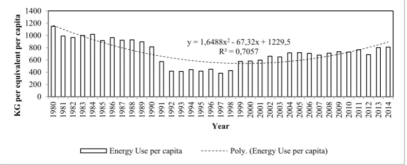
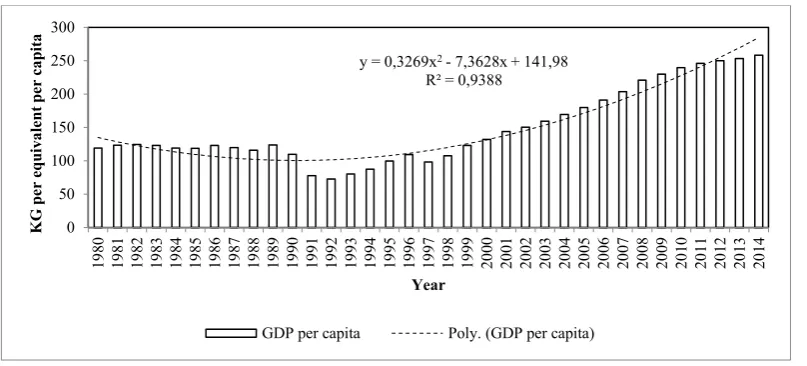
There has been a steady increase in energy consumption per capita and per capita income, at least since 1997 (see Figures 1 and 2). From 1946 to 1990, Albania was a Socialist People’s Republic, which acted economically like the People’s Republic of Korea. Like the Kim dynasty in North Korea, the Albanian long-term (1946–1986) dictator Enver Hoxha kept the planned economy running more or less in autarky at least since 1978. The political and economic collapse of the system in 1991 coincided with the breakdown of the Soviet Union and the dissolution of the Socialist Federal Republic Yugoslavia. The 1990s were a period of political and economic transition, which was characterized by political and social unrest and a very slow economic recovery with bitter setbacks resulting from the economic downturn associated with the collapse of the planning economy (GDP growth in 1990 and 1991 was -11 % and -29 %, respectively) (World Bank, 2017). The current (2016) industrial structure is characterized by a strong service and agricultural sector, contributing about 53 % and 23 %, respectively, to Albania’s value added, and 40 % and 42 %, respectively to employment. The Albanian energy sector is also very specific because nearly all electricity consumed is produced by hydropower or imported. Albania imports on average 10 % of its electricity (Ebinger, 2010) due to fluctuations in the rainfall on which hydropower depends and due to losses in the distribution system. Both effects have caused power shortages and outages in the past, for instance, in the dry year of 2007 when the average duration of the daily power outage was 3.4 hours (Bidaj et al., 2015). The yearly production ranged between 2788 GWh (2007) and 5895 GWh (2015). The dependence of the electricity sector on climate causes some challenges for the future. On the one hand, with an average increasing temperature caused by the climate change, the rainfall is expected to become scarcer in Albania. On the other hand, the electricity consumption per capita, although still relatively low with 2,500 kWh per year/capita (Bidaj et al., 2015), has quintupled since 1991. Because of this and a doubling of the total energy consumption since
1992, Albania imports between 14 % (2014) to 53 % (2002) of its total energy. According to Bidaj et al (2015), the electricity consumption is mainly by households (54 % of total electricity consumption), followed by the service sector (23 %), industry (20 %) and agriculture (1 %).
In 2012, half of the household’s energy demand was caused by heating (22 %) or by heating of water (23 %) (Bidaj et al., 2015). Moreover, all imported oil is used for transportation, and the gas imports are mostly demanded by the service sector including tourism.
The share of renewable energy was between 12 % (2007) and 31 % (2010). Because of the huge technical and non-technical losses of electricity, the Albanian government sold the distribution infrastructure company of the state-owned and biggest producer of electricity KESh to the Czech electricity giant CEZ. However, the partnership between the private shareholders and the government endured from 2010 to 2013 and eventually was settled via arbitration (Ali, 2015).
Since 2014, the World Bank has supported the government financially and technically to reform the Albanian electricity market (World Bank, 2014). The intention was to reduce electricity losses from 44 % in 2013 to 16 % in 2019, and to stabilize the financial situation of the Albanian electricity sector. Besides technical improvements, the World Bank plan is based on a hike of the electricity price from 9.5 Albanian Lek (ALL)/KWh in 2012 to 11.5 ALL/KWh in 2022 and to 13.5 ALL/KWh in the long-run, to get the electricity sector profitable. Simultaneously, the World Bank required the abolishment of the subsidized price of 7.7 ALL/kWh for the first 300 KWh of each household (Ali, 2015).
Against these developments, the study aims to contribute to the energy-growth literature by examining the effect of energy consumption in Albania using multiple estimation methods. The set-up of the paper is as follows. In Section 2, we provide a brief review of the energy-growth literature. In Section 3, we discuss the model and framework, followed by the results in Section 4. Lastly, in Section 5, some concluding remarks follow.
Figure 1. Energy Consumption. Source: World Bank (2018)
y = 1,6488x2- 67,32x + 1229,5
R² = 0,7057
0 200 400 600 800 1000 1200 1400 19 80 19 81 19 82 19 83 19 84 19 85 19 86 19 87 19 88 19 89 19 90 19 91 19 92 19 93 19 94 19 95 19 96 19 97 19 98 19 99 20 00 20 01 20 02 20 03 20 04 20 05 20 06 20 07 20 08 20 09 20 10 20 11 20 12 20 13 20 14 KG p er e qu iv al en t p er c ap it a Year
Figure 2. GDP per Capita. Source: World Bank (2017)
Literature Review
This section provides a brief survey of economic growth and energy consumption literature. The neo-classical and new growth theories are discussed. The energy consumption-growth nexus is summarized based on Payne’s (2010) four hypotheses. The growth hypothesis notes a unidirectional causality from energy consumption to economic growth; the conservation hypothesis notes a unidirectional causality from economic growth to energy consumption; the feedback hypothesis asserts a bi-directional causality; and the neutrality hypothesis implies that no relationship exists between energy consumption and economic growth.
Neo-Classical and New Growth Theory
Neo-classical growth theory of Solow (1956) asserts that exogenous technical progress is the only determinant of long run growth. Capital accumulation produces transitionary growth in excess of the steady state growth rates and the growth rates converge monotonically to the constant steady state growth rates over the process of many decades. Mankiw
et al.’s (1992) extension includes human capital as a shift and
variable Senhadji (2000) uses a growth accounting approach to show a way to estimate the determinants of productivity growth within a single equation framework.
The new growth theory was popularized by Romer (1986; 1990) through a series of papers which endogenize Solow’s total factor productivity. Many models of endogenous growth have been proposed because almost any factor hypothesized to influence productivity can be modelled within the complex system of equations describing each model. Most endogenous models work through positive externalities and are known for their micro foundations and optimizing agent framework. Additionally, the new growth theory can be considered as nested within the exogenous growth models and hence extensions of the Solow (1956) model based on new growth theory (Rao, 2010).
Energy-Growth Nexus
The energy-growth nexus summarized by Payne (2010) and Ozturk (2010) highlights four plausible causality directions. Countries for which the growth hypothesis is confirmed are: Philippines (Yu & Choi, 1985), Japan (Erol & Yu, 1987), the USA (Stern, 1993; 2000; Bowden & Payne,
2009), India and Indonesia (Masih & Masih, 1996), Singapore (Glasure & Lee, 1998), Turkey, France, Germany (Soytas & Sari, 2003; Altinay & Karagol, 2005), China (Soytas & Sari, 2003; Yuan et al., 2007), Benin, Congo, Tunisia (Wolde-Rufael, 2004; 2006), Tanzania, South Africa, Kenya (Odhiambo, 2009; Kumar & Kumar, 2013a; Kumar et al., 2015b), Nigeria (Akinlo, 2009), Lebanon (Abosedra et al., 2009), Gibraltar (Kumar et al., 2015a), Belgium, Spain (Omri et al., 2015), Malaysia (Azam et al., 2015), G7 countries (Bilgili & Ozturk, 2015), Denmark, Norway, Finland and Sweden (Hamit-Haggar, 2016; Irandoust, 2016), 20 European countries (dos-Santos-Gaspar, Marques, & Fuinhas, 2017), and 10 oil exporting countries (Hasanov, Bulut, & Suleymanov, 2017).
There are some studies which confirm the conservation hypothesis for certain countries. Among these countries are: the USA (Kraft & Kraft, 1978; Abosedra & Baghestani, 1989; Menyah & Rufael, 2010), India (Yu & Choi, 1985; Ghosh, 2002), West Germany (Erol & Yu, 1987), Indonesia and Thailand (Masih & Masih, 1996; Yoo 2006; Yoo & Kim, 2006), Korea and Italy (Oh & Lee, 2001a; Soytas & Sari, 2003), Australia (Narayan & Smyth, 2005), France, Japan (Lee, 2006), Congo (DRC) (Odhiambo, 2009), China (Zhang, 2009), Albania, Bulgaria, Hungary, Romania (Kumar et al., 2014a), Canada, Netherlands and Sweden (Omri et al., 2015; Kyophilavong et al., 2015),
Countries for which a bi-directional causality between energy and economic growth is confirmed are: Japan, Italy (Erol & Yu, 1987), Taiwan (Hwang & Gum, 1992), Pakistan (Masih & Masih, 1996), Tanzania, Nigeria (Ebohon, 1996), South Korea, Singapore (Glasure & Lee, 1998; Oh & Lee, 2004b), Philippines, Thailand (Asafu-Adjaye, 2000), Greece (Hondroyiannis et al., 2002), Argentina (Soytas & Sari, 2003), Canada (Ghali & El-Sakka, 2004), the USA (Lee, 2006), Malaysia (Tang, 2008), Egypt, Gabon, Morocco (Wolde-Rufael, 2006), Korea, Malaysia, Singapore (Yoo, 2005, 2006), Venezuela, Burkina Faso, Portugal (Yoo & Kwak, 2010; Shahbaz et al., 2011), Nasreen and Anwar (2014) for 15 Asian countries, China (Bloch et al., 2015; Bhattacharya et al., 2015), Argentina, Brazil, France (Omri
et al., 2015), Indonesia (Azam et al. (2015), MENA
countries (Kahia, Aissa, & Lanouar, 2017), Balkan countries (Kocak & Sarkgunesi, 2017), and 17 European countries (Zortuk & Karacan, 2018).
y = 0,3269x2- 7,3628x + 141,98
R² = 0,9388
0 50 100 150 200 250 300 19 80 19 81 19 82 19 83 19 84 19 85 19 86 19 87 19 88 19 89 19 90 19 91 19 92 19 93 19 94 19 95 19 96 19 97 19 98 19 99 20 00 20 01 20 02 20 03 20 04 20 05 20 06 20 07 20 08 20 09 20 10 20 11 20 12 20 13 20 14 KG p er e qu iv al en t p er c ap it a Year
On the other hand, some studies note support for neutrality hypothesis. Among these include countries like: Kenya, South Africa, Sudan and the USA (Akarca & Long, 1980; Yu & Hwang, 1984; Yu & Choi, 1985), Malaysia, Singapore, Philippines, South Korea (Masih & Masih, 1996; Glasure & Lee, 1998), Indonesia, India, Turkey (Asafu-Adjaye, 2000; Altinay & Karagol, 2004), the UK, Germany, Sweden, Algeria, Congo Republic (Lee, 2006; Wolde-Rufael, 2006), Finland, Hungary, India, Japan, Switzerland (Omri et al., 2015), Thailand (Azam et al., 2015), 42 Sub Saharan African countries (Menegaki & Tugcu, 2017), USA (Menegaki & Tiwari, 2017) and Turkey (Bulut & Muratoglu, 2018).
Few things are clear from the literature. The effect of energy on economic growth and the direction causality differs for countries and regions, because of the differences in the sample size, model specification, methodology and the measurement variables used for energy and economic growth. Also, lesser focus is on the magnitude (elasticity) effects, mainly because estimating elasticity is not straight forward. The model specification requires a well-established theory and the model needs to minimise the problem of misspecification.
Moreover, some studies use the augmented Solow (1956) framework for model specification. For small samples, estimation methods like the autoregressive distributed lag (ARDL) procedure of Pesaran, Shin and Smith (2001) is recommended (Odhiambo, 2009) to minimise endogeneity. Additionally, accounting for structural breaks, and the magnitude effects may provide important policy insights (Smyth & Narayan, 2014).
Energy Growth Nexus in Albania
Ozturk and Acaravci (2010) examine the causal effect of energy consumption on real output in Albania over 1980-2006 using the ARDL method. The authors conclude that there is no long run relationship between energy consumption and per capita output. Additionally, they find no evidence of any causality. Kumar et al. (2014) apply an extended Solow (1956) framework over 1980–2011. They use the ARDL method and examine causality using the Toda and Yamamoto (1995) procedure. The capital stock elasticity is 0.55 and the elasticity of income with respect to energy consumption is 0.07. The causality results indicate a unidirectional causation from output per worker to energy consumption per worker. Kumar et al. (2017) re-examine the energy-growth relationship for 12 Balkan nations. For Albania, they find capital stock share is 0.22 and the energy elasticity is 0.29, and like Kumar et al. (2014), confirm conservation hypothesis.
From these studies (Ozturk & Acaravci, 2010; Kumar et al., 2014; Kumar et al., 2017), a few points emerge. First, a sound theoretical framework deliver more plausible outcomes of the effect of energy consumption on output; second, there is a contention on the strength of the effect of energy on output; and third, conservation hypothesis is shown to exist (Kumar et al., 2014; Kumar et al., 2017). However, these studies use a single estimation method. Also, Kumar et al. (2017) identify structural breaks using the single break tests of Zivot and Andrews (1992) and Perron (1997). We apply multiple break tests and use more than one method of estimation to obtain robust and consistent results.
Data & Method
Model
We use an augmented Cobb-Douglas production function similar to the Solow (1956) which is applied by Sturm (1998) and others (Rao 2010; Rao & Hassan, 2012; Jawaid & Raza, 2016; Hassan, Chowdhury & Bhuyan 2016; Park & Seo, 2016; Kumar et al., 2017; Kumar et al., 2018a, b). The model assumes Hicks neutral technical progress, where output per worker, ytis given as:
yt= Atktα 0 < 𝛼 < 1 (1)
where 𝐴𝑡 is the stock of technology and knowledge, 𝑘𝑡
is per worker capital stock 𝛼 is the capital share and with constant returns to scale assumption. The model assumes that the evolution of technology is given by:
Φt= A0egt (2)
where 𝐴0is the initial stock of technology and 𝑡 is time
trend. We introduce energy consumption per worker (𝑒𝑛𝑔) as a shift variable (Rao, 2010).
Ψt= f(eng) = engtϑ (3)
Where ϑ > 0 represents the elasticity of energy consumption per worker, hence:
At= ΦtΨt= A0egtengtϑ (4)
Finally, including this information in (1), we arrive at:
yt= A0egtengtϑktα (5)
For estimation we take the log of (5) and add an error term:
lnyt= lnA0+ gt + αlnkt+ ϑlnengt+ ut (6)
where yt is real GDP per worker, kt is real capital stock
per worker, engt is energy consumption per worker, 𝜙 is the
constant term, t is the time trend and ut is the error term.
Lag Estimate, Long Run & Dynamic Estimation
Lags are suitable to model the effects of persistence and inertia, and they can capture institutional and behavioural characteristics. Hence, following Stauvermann et al. (2016), we specify following lagged equation:
lnyt= β0+ β1T + ∑pi=11 γ1iln yt−i+ ∑pi=02 δ1iln kt−i+
∑pi=03 θ1iln engt−i+ εt (7)
Using (7), we can derive the long run coefficients in (6) as:
𝑙𝑛𝐴0=
𝛽0
1 − ∑𝑝𝑖=11 𝛾1𝑖
; 𝑔 = 𝛽1 1 − ∑𝑝𝑖=11 𝛾1𝑖
; 𝛼 = ∑ 𝛿1𝑖
𝑝2
𝑖=0
1 − ∑𝑝𝑖=11 𝛾1𝑖
; 𝜗
= ∑ 𝜃1𝑖
𝑝3
𝑖=0
1 − ∑𝑝𝑖=11 𝛾1𝑖
; 𝑢𝑡=
𝜀𝑡
1 − ∑𝑝𝑖=11 𝛾1𝑖
~𝑁(0, 𝜎2)
∆ ln yt= ∑pi=11 γ1iΔln yt−i+ ∑i=0p2 δ1iΔln kt−i+ ∑pi=03 θ1iΔln engt−i−
𝜆[lnyt− lnA0− gt − αlnkt− ϑlnengt] + εt (8)
Equation (8) is consistent with many estimation methods such as the general to specific (GETS) (Hendry, 1987), the Johansen Maximum Likelihood (Johansen, 1988; 1991) and ARDL approach (Pesaran et al., 2001). Moreover, equation (8) is also consistent with the data generating process and cointegration theory. Additionally, the one-step estimation avoids the small sample bias present in the Engle and Granger (1987) two-step approach. Estimates of equation (8) can be obtained by imposing steady state equilibrium restrictions on equation (8). Stability of equation 7 requires that the coefficient of ln yt−1 is between zero and positive unity. The
error correction term, which measures the speed of adjustment to the equilibrium, is equal to one minus this coefficient.
We use the ARDL approach (Pesaran, et al., 2001). Equation (8) is first estimated using the OLS technique and then the restrictions are applied to the lagged level variables. The advantages of the approach are that: (i) cointegration can be examined with the combination of stationary and non-stationary series, (ii) it is suitable for small samples, (iii) it minimizes endogeneity bias through its dynamic structure, and (iv) it does not require symmetry in lags for each explanatory variable.
Causality Analysis
The vector error correction method (VECM) is used to examine causality. Advantages of the VECM is that: (i) it is congruent with the data generation process, (ii) it handles the non-stationarity problems of time-series data, (iii) all variable are assumed to be endogenous, and (iv) it can be used to implement the Johansen’s cointegration test to identify the number of cointegrating vectors within the sample. Subsequently, the following vector error correction models are:
∆ ln yt= ϕ10+ ϑ10T + ∑pi=11 γ1iΔln yt−i+
∑pi=02 δ1iΔln kt−i+ ∑i=0p3 θ1iΔln engt−i− λ1ECT1,t−1+ ε1t (9)
∆ ln kt= ϕ20+ ϑ20T + ∑pi=11 γ2iΔln yt−i+
∑pi=02 δ2iΔln kt−i+ ∑i=0p3 θ2iΔln engt−i− λ2ECT2,t−1+ ε2t (10)
∆ ln engt= ϕ30+ ϑ30T + ∑pi=11 γ3iΔln yt−i+
∑pi=02 δ3iΔln kt−i+ ∑i=0p3 θ3iΔln engt−i− λ3ECT3,t−1+ εt (11)
The test of causality is a test of joint restrictions in equations 9-11. In equation (9), short run causality from
lnvist to lnyt and from lnkt to lnyt implies that θ1i∀i ≠ 0
and δ1i∀i ≠ 0; In equation (10) short run causality from
lnengt to lnkt and from lnyt to lnkt implies that θ2i∀i ≠ 0
and δ2i∀i ≠ 0; and in equation (11) short run causality from
lnkt to lnengt and from lnyt to lnengt implies that θ3i∀i ≠
0 and δ3i∀i ≠ 0. The long run joint causality depends on (i)
significance of the error correction term, (ii) the correct sign of the error correction term, and (ii) the number of cointegrating vectors in the system.
Results and Discussion
Data Sources
We use a total of 35 years of annual data over the periods 1980-2014.The data for real GDP is from 1980 to 2016, total population is from 1960 to 2016, labour force participation rate is from 1990 to 2016, gross fixed capital formation (%
of GDP) as a proxy investment is from 1980 to 2016, and energy consumption (kg of oil equivalent per capita) is from 1971 to 2014. The data is sourced from the World Development Indicators and Global Development Finance database (World Bank, 2017). Real GDP and gross fixed capital formation are measured in constant 1996 Albanian Lek (ALL). The physical capital stock series is constructed using the perpetual inventory method where the initial capital stock is set to 1.5 times the 1962 real GDP. The depreciation rate is assumed at 5 percent. The labour stock is computed as the average of the participation rate (averaged at 58.7 % from 1990 to 2016) multiplied by the respective year’s population. Given the different starting points of the series, for consistency, the sample from 1980 to 2014 is used for the analysis.
Descriptive Statistics
Table 1 presents the descriptive statistics and correlation matrix.
Table 1
Descriptive Statistics and Correlation Matrix 1980–2014
Statistics 𝐥𝐧𝐲𝐭 𝐥𝐧𝐤𝐭 𝐥𝐧𝐞𝐧𝐠𝐭
Panel a: descriptive statistics
Mean 12.37 13.51 7.07
Median 12.25 13.35 7.10
Maximum 12.99 14.26 7.58
Minimum 11.73 12.63 6.48
Standard deviation 0.36 0.44 0.31
Skewness 0.27 0.21 -0.44
Kurtosis 2.12 2.20 2.17
Normality 1.55 1.18 2.11
[0.50] [0.55] [0.35]
Panel b: correlation matrix
lnyt
1.00 --
lnkt
0.82***
[<0.01]
1.00 --
lnengt
0.36**
[0.03]
-0.12
[0.51] 1.00--
Notes: [ ] contains p-value. *** and ** indicates significance at 1 % and 5 % level.
The (natural) log values of kt and engt are positively
correlated with yt. Moreover, based on a skewness-kurtosis
(Jarque-Bera) test, the variables are normally distributed.
Unit Root
Table 2
Unit Root
Variables
ADF test statistic PP test statistic Level Difference 1st Level Difference 1st
lnyt -2.06 (0) [0.54] -4.40 (0)
***
[<0.01]
-1.56 (1) [0.79]
-3.75 (0)***
[<0.01]
lnkt
-3.00 (0) [0.15]
-5.22 (8)***
[<0.01]
-2.14 (3) [0.51]
-2.26 (2)**
[0.02]
lnengt
-1.22 (0) [0.88]
-4.49 (0)***
[<0.01]
-1.38 (2) [0.85]
-4.49 (1)***
[<0.01]
Notes: Lag used in ADF and Bandwidth in PP are indicated in round parenthesis and determined using the Schwarz criterion. P value reported in square parenthesis, *** - stationary at 1 percent, ** - stationary at 5 %,
null hypothesis – series has unit root, test conducted with constant and trend; test statistic reported is t-statistic for ADF and adjusted t-statistic for PP test.
Lag Length Tests
Lag length tests (Table 3) are based on a number of information criterions. The maximum lags indicated by the SC criteria are 3. Setting the lags to 3 yields the optimum lag combination of ARDL (1, 2, 1).1
Table 3
Lag Selection Tests
Lag LL LR FPE AIC SC HQ
1 159.97 -- 1.2 x 10⁻⁸ -9.74 -9.32 -9.60
2 183.41 37.81 4.7 x 10⁻⁹ -10.67 -9.83*** -10.40
3 195.76 17.52*** 3.9 x 10⁻⁹*** -10.88*** -9.64 -10.48***
4 201.88 7.51 5.1 x 10⁻⁹ -10.70 -9.03 -10.16
Notes: LL – log likelihood; LR – likelihood ratio; FPE – Final prediction error; AIC – Akaike information criterion, SC – Schwarz criterion, HQ – Hannan-Quinn criterion, -- not applicable, *** indicates optimal lag length at 5 %.
Structural Breaks
Structural breaks are examined using the Bai and Perron (1998; 2003) multiple break test (Table 4). The advantages of this approach are: (i) the existence of multiple breaks can be identified which then can be used to analyse real events that characterize the break periods, and (ii) using breaks, regimes in the data can be identified and accounted for, thus improving the forecasting ability of the model. Additionally, the responsiveness of the dependent variable due to the structural breaks can be ascertained. This can be information for policy makers (Stauvermann et al., 2016; Ahmad and Aworinde, 2015 and Das et al., 2014).
Table 4
Break Test
Null hypothesis Scaled F-statistic Critical Value
0 vs. 1 51.35*** 8.58
1 vs. 2 13.86*** 10.13
2 vs. 3 3.56 11.14
Break dates: 1995; 2007
Source: estimated in Eviews 9, critical value from Bai-Perron (1998; 2003), *** - significant at 5 %
Cointegration Tests
We perform three tests of cointegration: (i) the ARDL procedure of Pesaran et al. (2001) (Table 5a), (ii) the trace and maximum eigenvalue tests of Johansen (1988) and Johansen and Juselius (1991) (Table 5b) and (iii) the residual based cointegration tests of Engle and Granger (1987), and Phillips-Ouliaris (1990) (Table 5c). The tests (ii) and (iii) are performed to examine the consistency of the results with respect to the results obtained from the ARDL method.
Table 5a
Bounds test – ARDL (1,2,1)
Model F-Statistic
lnyt|lnkt; lnengt; B1; B2 5.66**
lnyt|lnkt; lnengt 2.77 Critical Value Bounds
Significance I(0) Bound I(1) Bound
10 % 3.17 4.14
5 % 3.79 4.85
1 % 5.15 6.36
Note: *** indicates rejection of the given number of cointegrating vectors
1 Using a maximum of 2 or 4 lags gave the same optimal lag combination
of ARDL (1,2,1).
Table 5b
Johansen’s Cointegration Test
Hypothesized Eigen value Trace 5 % CV value P- Eigen Max- 5 % CV value P-No. of CE(s) Statistic Statistic
lnyt|lnkt, lnengt, B1, B2
None 0.57 34.56*** 29.79 <0.01 27.05*** 21.13 <0.01
At most 1 0.20 7.51 15.49 0.52 7.50 14.26 0.43 At most 2 7.41x 10⁻⁵ 0.01 3.84 0.95 0.01 3.84 0.96
lnyt|lnkt, lnengt
None 0.46 36.02*** 29.79 <0.01 20.62 21.13 0.06
At most 1 0.32 15.39 15.49 0.06 12.34 14.26 0.09 At most 2 0.09 3.049 3.84 0.08 3.049 3.84 0.08
Note: *** indicates rejection of the given number of cointegrating vectors.
Table 5c
Residual Based Tests
Variable
Engle-Granger Phillips-Ouliaris Tau
statistic Z statistic
Tau statistic
Z statistic
Cointegrating residual
-4.44B
[0.02]
-25.45B
[0.02]
-4.41B
[0.02]
-22.38B
[0.04] Note: B – cointegration at 5%.
The cointegrating relationship between lnyt, lnkt and
lnengt (specified in equation 6) is accepted at the 5 percent
level after the inclusion of structural breaks (Table 5a). Moreover, cointegration is also confirmed in Tables 5b and 5c.
Long & Short Run Estimates
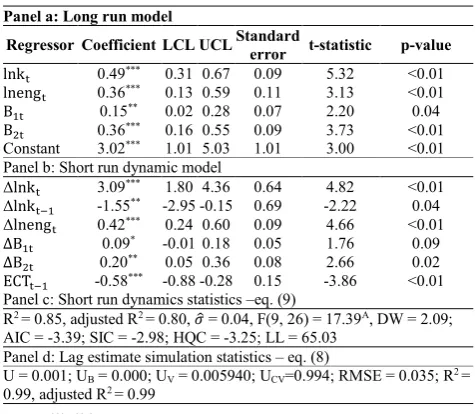
The long and short run results based on the ARDL (1,2,1) are selected on the basis of the Akaike information criteria (Table 6).
Table 6
Estimated Long & Short Run Models – ARDL (1,2,1)
Panel a: Long run model
Regressor Coefficient LCL UCL Standard error t-statistic p-value
lnkt 0.49*** 0.31 0.67 0.09 5.32 <0.01
lnengt 0.36*** 0.13 0.59 0.11 3.13 <0.01
B1t 0.15** 0.02 0.28 0.07 2.20 0.04
B2t 0.36*** 0.16 0.55 0.09 3.73 <0.01
Constant 3.02*** 1.01 5.03 1.01 3.00 <0.01
Panel b: Short run dynamic model
Δlnkt 3.09*** 1.80 4.36 0.64 4.82 <0.01
Δlnkt−1 -1.55** -2.95 -0.15 0.69 -2.22 0.04
Δlnengt 0.42*** 0.24 0.60 0.09 4.66 <0.01
∆B1t 0.09* -0.01 0.18 0.05 1.76 0.09
∆B2t 0.20** 0.05 0.36 0.08 2.66 0.02
ECTt−1 -0.58*** -0.88 -0.28 0.15 -3.86 <0.01
Panel c: Short run dynamics statistics –eq. (9)
R2 = 0.85, adjusted R2 = 0.80, 𝜎̂ = 0.04, F(9, 26) = 17.39A, DW = 2.09;
AIC = -3.39; SIC = -2.98; HQC = -3.25; LL = 65.03 Panel d: Lag estimate simulation statistics – eq. (8)
U = 0.001; UB = 0.000; UV = 0.005940; UCV=0.994; RMSE = 0.035; R2 =
0.99, adjusted R2 = 0.99
Notes: *** ,**,* - significance at 1,5,10 percent levels, LCL & UCL- 5 %
lower and upper confidence interval, U – Theil’s inequality coefficient, UB
, UC – bias and variance proportions of U, UCV – unsystematic component
As noted from Table 6, the cointegrating coefficient of lnktis estimated at 0.49, which indicates that in the long run,
a 1 % increase in kt increases yt on average by 0.49 %, ceteris
paribus. This differs from Kumar et al. (2017) where the
capital elasticity is noted at 0.22 and is closer to Kumar et al. (2014) who estimate an elasticity of 0.55. According to our results, the capital share exceeds the stylized value of one third, and this is expected for developing and transitional countries where the marginal productivity of capital is notably higher (Kumar & Stauvermann, 2014). In terms of the lower and upper confidence limits, we note that the coefficient of lnkt ranges from 0.30 to 0.67 at the 5 % level of significance.
The coefficient of lnengt is 0.36 which implies that a 1 %
increase in per worker energy consumption increases yt by
0.36 %. Kumar et al. (2017) and Kumar et al. (2014) note the share to be 0.29 and 0.07, respectively. Also, in our study, the two break periods have a positive association with real output.
In the short-run (Panel b, Table 6), the capital stock (investment) has a significant and positive association with growth (Δlnkt+Δlnkt−1= 1.54), whereas Kumar et al.
(2014) and Kumar et al. (2017) find this to be at 1.92 and 2.49, respectively. The coefficient of energy consumption is positive and statistically significant (Δlnengt = 0.42) which
implies that a 1 % increase in energy consumption increase growth of per worker output by 0.42 %, ceteris paribus. Kumar et al. (2014) and Kumar et al. (2017) note a slightly lower short-run magnitude of at 0.37 and 0.25, respectively. On ECTt−1 , the coefficient is negative (-0.5809) and
significant at the 1 % level. This indicates that on average, following exogenous shocks, the convergence to long run equilibrium takes approximately 1.7 years, ceteris paribus.
ARDL Diagnostics
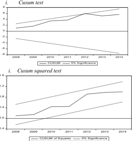
We use the Ramsey reset test to detect omitted variables and incorrect functional form and the Breusch-Godfrey test to detect residual autocorrelation. Additional tests used are the Breusch-Pagan-Godfrey test of heteroscedasticity, Jarque-Bera normality test, and the Durbin-Wu-Hausman test of regressor endogeneity. The parameter stability is examined from the CUSUM and CUSUMQ (CUSUM squared) plots. As noted from the statistics in Table 7 and Figure 3, the model passes the diagnostic and parameter stability tests. Moreover, the results of the Durbin-Wu-Hausman test for endogeneity coincides with the trace and maximum Eigen value tests.
Table 7
ARDL (1,2,1) Diagnostic Tests
Test Null hypothesis Test Version 1
Ramsey
RESET H0: No omitted variables F(1,23) = 0.06
0.81
Breusch-Godfrey Hautocorrelation 0: No residual χ2(2) = 0.40 0.82
Breusch-Pagan-Godfrey H0: Homoscedasticity χ2(8) = 11.02
0.20
Jarque-Bera H0: Residual normality χ2(1) = 0.28 0.87
Durbin-Wu-Hausman
H0: Joint Regressor
exogeneity χ2(6) = 1.90
0.93
i. Cusum test
-8 -6 -4 -2 0 2 4 6 8
2008 2009 2010 2011 2012 2013 2014
CUSUM 5% Significance
i. Cusum squared test
-0.4 0.0 0.4 0.8 1.2 1.6
2008 2009 2010 2011 2012 2013 2014
CUSUM of Squares 5% Significance
Figure 3. ARDL Cusum stability tests at 5 %.
Causality Tests
The results of the VECM satisfy the statistical conditions of no residual autocorrelation, homoskedasticity, residual normality and stability as noted by the inverse root plot (Figure 4).
Table 8
VECM Causality Results
Excluded Test Statistic P Value
Panel a: causality test Dependent variable: ∆lnyt
∆lnvist 𝜒2(2) =1.08 0.58
∆lnengt 𝜒2(2) = 0.25 0.88
Joint 𝜒2(4) = 1.67 0.79
Dependent variable: ∆lnkt
∆lnyt 𝜒2(2) = 6.40** 0.04
∆lnengt 𝜒2(2) = 1.77 0.41
Joint 𝜒2(4) =6.69 0.15
Dependent variable: ∆lnengt
∆lnyt 𝜒2(2) =10.13*** 0.01
∆lnkt 𝜒2(2) = 0.32 0.85
Joint 𝜒2(4) = 12.42** 0.015
Panel b: Implied long run elasticity– JML
Variable Coefficient Standard Error T-Statistic P Value
lnkt 0.515111A 0.082 -6.254 <0.01
lnengt 0.499224A 0.137 -3.640 <0.01
Panel c. VECM diagnostics
SC: χ2(9) = 5.83 [0.75]; HC: χ2(96) = 104.10 [0.2687]; RN:
χ2(1) = 8.277[0.22]; R2 = 0.4950; adjusted R2=0.28; 𝜎̂ = 0.08, AIC =
-2.05; SIC = -1.59; F = 2.40***; LL = 42.85
Notes: *** and ** indicate significance at 1% and 5%, respectively. SC –
serial correlation, HC – heteroskedasticity, RN – residual normality, p value in square parenthesis and diagnostic test degrees of freedom in round parenthesis in panel c, heteroskedasticity test is based on White’s test without cross products, LL – log likelihood.
Causality results based on 𝜒2 test are presented in Table
8. We note a unidirectional causality from ∆lnytto ∆lnengt,
and a unidirectional causality ∆lnytto ∆lnkt. The causality
-1.5 -1.0 -0.5 0.0 0.5 1.0 1.5
-1.5 -1.0 -0.5 0.0 0.5 1.0 1.5
Inverse Roots of AR Characteristic Polynomial
Figure 4. VECM IR stability plot at 5 %
Robustness Tests
For robustness tests, the long-run relationship is estimated using the dynamic OLS (DOLS) procedure (Saikkonen, 1992; Stock & Watson, 1993). To remove long run serial correlation within the error term, the DOLS method constructs an asymptotically efficient estimator by augmenting the cointegrating equation with leads and lags of the differenced explanatory variables. The resulting error term is orthogonal to the entire history of the stochastic regressor innovations.
Table 9
Estimated Long-Run Model – DOLS
Variable Coefficient LCL UCL standard error statistic t- p-value
𝑙𝑛𝑘𝑡 0.49*** 0.36 0.61 0.06 7.59 <0.01
𝑙𝑛𝑒𝑛𝑔𝑡 0.43*** 0.26 0.60 0.08 5.00 <0.01
𝐵1 0.16*** 0.05 0.27 0.05 2.91 <0.01
𝐵2 0.32*** 0.18 0.47 0.07 4.38 <0.01
Constant 2.51*** 1.09 3.93 0.71 3.54 <0.01
R2 = 0.99, adjusted R2 = 0.99,𝜎̂ = 0.05; 𝜒
𝑅𝑁2 (1) = 0.47 [0.79]; LQ(1) =
0.69 [ 0.46] 𝑉𝐼𝐹̅̅̅̅̅ = 7.28; LC = 0.104 [0.20]
Notes: *** indicate significance at 1%; RN – residual normality; LQ –
Ljung-box serial correlation statistic, degrees of freedom in 𝜒2 and lags
used in LQ indicated in ( ) and p-value for these tests in [ ], LC = Hansen instability test.
The DOLS result (Table 9) is consistent with the results reported using the ARDL and the JML procedure. Therefore, the capital share is between 0.48 and 0.51, and the energy elasticity is between 0.36 and 0.49.
Instrumental Variables (IV) and GMM Estimates Except for the Johansen’s method which utilizes the maximum likelihood estimators, the other methods use the ordinary least squares (OLS) estimators. The latter may produce biased and inconsistent results in the presence of endogeneity and/or inaccurate model specification. Therefore, we check our estimates by applying the IV and GMM estimates. The IV and GMM estimates are presented in Table 10 and 11, respectively. As noted, the results obtained are consistent with the previous estimation methods, free from endogeneity bias, serial correlation, and heteroscedasticity, and has the correct functional form with its residuals being normally distributed.
Table 10
Estimated Long-Run Model – IV
Variable Coefficient LCL UCL standard error t-statistic value
p-𝑙𝑛𝑘𝑡 0.42*** 0.22 0.62 0.10 4.12 <0.01
𝑙𝑛𝑒𝑛𝑔𝑡 0.58*** 0.49 0.67 0.05 12.65 <0.01
𝐵1 0.30*** 0.23 0.38 0.04 8.21 <0.01
𝐵2 0.45*** 0.26 0.65 0.09 4.62 <0.01
Constant 2.36* -0.19 4.91 1.28 1.85 0.08
R2 = 0.98, adjusted R2 = 0.98 𝜎̂ = 0.05; 𝜒 𝐸𝑁
2 (2) = 3.68 [0.15];
𝐹𝑅𝑅(1, 24) = 1.97 [0.17]; 𝜒𝑆𝐶2(1) = 0.85 [0.35]; 𝜒𝐻𝑇2 (2) = 2.10
[0.3490]; 𝐴𝑅𝑁2 (1) = 0.71 [0.55]
Notes: *** and * indicate significance at 1 % and 10 %, respectively,
EN – endogeneity Hausman test; RR – Ramsey RESET; SC – serial correlation; HT – heteroskedasticity; RN – residual normality
Table 11
Estimated Long-Run Model – GMM
Variable Coefficient LCL UCL standard error t-statistic p-value
𝑙𝑛𝑘𝑡 0.43*** 0.36 0.50 0.04 11.83 <0.01
𝑙𝑛𝑒𝑛𝑔𝑡 0.58*** 0.53 0.63 0.03 22.77 <0.01
𝐵1 0.30*** 0.27 0.34 0.02 19.20 <0.01
𝐵2 0.45*** 0.38 0.51 0.03 13.95 <0.01
Constant 2.27*** 1.61 2.94 0.33 6.83 <0.01
R2 = 0.98, adjusted R2 = 0.98,𝜎̂ = 0.05
Notes: *** indicate significance at 1%
Conclusion
In this study, we examine the energy-growth nexus in the case of Albania over 1980–2014 using the ARDL approach of Pesaran et al. (2001) and the JML procedure of Johansen (1988; 1991). Causality is tested using the VECM technique. The existence of a single cointegrating vector is noted. Other methods such as DOLS, IV and GMM procedures also provide consistent results. The average capital share is 0.49 and the elasticity of per worker energy consumption is 0.35. The causality results support the conservation hypothesis for Albania, similar to Kumar et al. (2014) and Kumar et al. (2017).
Some policy implications can be drawn from the results. It is clear that energy consumption is a consequence of economic activity and important facilitating further economic activity. Our results are also consistent with O’Brien et al. (2017), who argue that 15 % of all firms in Albania consider (lack if) electricity as the main constraint in doing business. The World Bank (2017) has ranked Albania in terms of doing business at 157 (out of 190) and in terms of the reliability of electricity, at zero (in the range of zero and eight). The European and Central Asian countries have received on average a value of 5 and high income OECD countries of 7. Under these circumstances, it is not much surprising that Albania’s industry sector is not well developed.
One of the main obstacles of Albania’s energy sector is the missing reliability and low profitability of the electricity sector. Bidaj et al (2015) estimate that 29 % to 52 % of the total electricity supply is lost due to technical and non-technical (theft and unpaid bills) reasons. Ali (2015) states that the technical losses accounted for 16 % of the total electricity supply in 2014.
depends on the rainfall, it is recommended to incentivize private investments in renewable electricity production like solar panels or wind turbines. It should be clear, that all possible foreign investments even in the potential profitable emerging sector like tourism are nearly stalled if the energy supply is not reliable. Noting that Albania is an energy resource-abundant country, a key policy objective should be to transform the economy to become more efficient in energy use and productivity growth. A reliable energy supply is a precondition for the exploitation of other economic advantages such as the country’s low wage level to improve economic development.
The government should consider introducing a progressive electricity billing system for households, which can be adjusted according to the available water resources to
guarantee the electricity supply for firms. Such a progressive billing system will incentivize the purchase of energy-saving devices and solar panels, ensure the availability of electricity is at an affordable price, and ensure that electricity supply for companies are stable. Additionally, for effective and forward looking plans, the government will need to consider the effects of climate change on the rainfall in the coming decades. It is thus recommended that energy supply is diversified. Because of the relatively low electricity price, the option to use solar water heating panels seems to be economically viable. Also, there is a need to improve water management in the agricultural sector to cater for the water demand for irrigation purposes whilst supporting the energy sector in hot dry summers
.
Acknowledgement
The authors would like to thank the anonymous reviewers, the Editor-in-Chief and the editorial team of Engineering
Economics. Peter J. Stauvermann acknowledges thankfully the financial support of the Changwon National University
Research Fund in 2019. The usual disclaimer applies.
References
Abosedra, S., & Baghestani, H. (1989). New evidence on the causal relationship between United States energy consumption and gross national product. The Journal of Energy and Development, 14(2), 285–292.
Abosedra, S., Dah, A., & Ghosh, S. (2009). Electricity consumption and economic growth, the case of Lebanon. Applied
Energy, 86(4), 429–432. https://doi.org/10.1016/j.apenergy.2008.06.011
Ahmad, A. H., & Aworinde, O. B. (2015). Structural breaks and twin deficits hypothesis in African countries. Economic
Change and Restructuring, 48(1), 1–35. https://doi.org/10.1007/s10644-014-9154-2
Akarca, A. T., & Long, T. V. (1980). On the relationship between energy and GNP: a reexamination. The Journal of
Energy and Development, 5(2), 326–331.
Akinlo, A. E. (2009). Electricity consumption and economic growth in Nigeria: evidence from cointegration and co-feature analysis. Journal of Policy Modeling, 31(5), 681–693. https://doi.org/10.1016/j.jpolmod.2009.03.004 Ali, O. (2015). Revitalizing the Albanian Electricity Sector, Case study, Center for International Development, Harvard
University. https://albania.growthlab.cid.harvard.edu/blog/new-case-study-revitalizing-albanian-electricity-sector Altinay, G., & Karagol, E. (2004). Structural break, unit root, and the causality between energy consumption and GDP in
Turkey. Energy Economics, 26(6), 985–994. https://doi.org/10.1016/j.eneco.2004.07.001
Altinay, G., & Karagol, E. (2005). Electricity consumption and economic growth: evidence from Turkey. Energy
Economics, 27(6), 849–856. https://doi.org/10.1016/j.eneco.2005.07.002
Apergis, N., & Payne, J. E. (2010a). Renewable energy consumption and economic growth: evidence from a panel of OECD countries. Energy policy, 38(1), 656–660. https://doi.org/10.1016/j.enpol.2009.09.002
Apergis, N., & Payne, J. E. (2010b). Renewable energy consumption and growth in Eurasia. Energy Economics, 32(6), 1392–1397. https://doi.org/10.1016/j.eneco.2010.06.001
Apergis, N., & Payne, J. E. (2011a). The renewable energy consumption-growth nexus in Central America. Applied
Energy, 88(1), 343–347. https://doi.org/10.1016/j.apenergy.2010.07.013
Apergis, N., & Payne, J. E. (2011b). Renewable and non-renewable electricity consumption-growth nexus: evidence from emerging market economies. Applied Energy, 88(12), 5226–5230. https://doi.org/10.1016/j.apenergy.2011.06.041 Apergis, N., & Payne, J. E. (2012). Renewable and non-renewable energy consumption-growth nexus: Evidence from a
panel error correction model. Energy Economics, 34(3), 733–738. https://doi.org/10.1016/j.eneco.2011.04.007 Asafu-Adjaye, J. (2000). The relationship between energy consumption, energy prices and economic growth: time series
evidence from Asian developing countries. Energy Economics, 22(6), 615–625. https://doi.org/10.1016/S0140-9883(00)00050-5
Bai, J., & Perron, P. (1998). Estimating and testing linear models with multiple structural changes. Econometrica, 47–78. https://doi.org/10.2307/2998540
Bai, J., & Perron, P. (2003). Computation and analysis of multiple structural change models. Journal of applied
econometrics, 18(1), 1–22. https://doi.org/10.1002/jae.659
Bhattacharya, M., Rafiq, S., & Bhattacharya, S. (2015). The role of technology on the dynamics of coal consumption-economic growth: New evidence from China. Applied Energy, 154, 686–695. https://doi.org/10.1016/j. apenergy.2015.05.063
Bidaj, F., Alushaj, R., Prifti, L., & Chittum, A. (2015). Evaluation of the heating share of household electricity consumption using statistical analysis: a case study of Tirana, Albania. International Journal of Sustainable Energy
Planning and Management, 5, 3–14.
Bilgili, F., & Ozturk, I. (2015). Biomass energy and economic growth nexus in G7 countries: Evidence from dynamic panel data. Renewable and Sustainable Energy Reviews, 49, 132–138. https://doi.org/10.1016/j.rser.2015.04.098 Bloch, H., Rafiq, S., & Salim, R. (2015). Economic growth with coal, oil and renewable energy consumption in China:
Prospects for fuel substitution. Economic Modelling, 44, 104–115. https://doi.org/10.1016/j.econmod.2014.09.017 Bowden, N., & Payne, J. E. (2009). The causal relationship between US energy consumption and real output: a
disaggregated analysis. Journal of Policy Modeling, 31(2), 180–188. https://doi.org/10.1016/j.jpolmod.2008.09.001 Bowden, N., & Payne, J. E. (2010). Sectoral analysis of the causal relationship between renewable and non-renewable energy consumption and real output in the US. Energy Sources, Part B: Economics, Planning, and Policy, 5(4), 400– 408. https://doi.org/10.1080/15567240802534250
Bulut, U., & Muratoglu, G. (2018). Renewable energy in Turkey: Great potential, low but increasing utilization, and an empirical analysis on renewable energy-growth nexus. Energy Policy, 123, 240–250. https://doi.org/10. 1016/j.enpol.2018.08.057
Cheung, Y. W., & Lai, K. S. (1995). Lag Order and Critical Values of a Modified Dickey‐Fuller Test. Oxford Bulletin of
Economics and Statistics, 57(3), 411–419. https://doi.org/10.1111/j.1468-0084.1995.mp57003008.x
dos Santos Gaspar, J., Marques, A. C., & Fuinhas, J. A. (2017). The traditional energy-growth nexus: A comparison between sustainable development and economic growth approaches. Ecological Indicators, 75, 286–296. https://doi.org/10.1016/j.ecolind.2016.12.048
Ebinger, J. (2010). Albania's Energy Sector: Vulnerable to Climate Change, Europe & Central Asia Knowledge Brief 29, World Bank.
Ebohon, O. J. (1996). Energy, economic growth and causality in developing countries: a case study of Tanzania and Nigeria. Energy Policy, 24(5), 447–453. https://doi.org/10.1016/0301-4215(96)00027-4
Engle, R. F., & Granger, C. W. (1987). Co-integration and error correction: representation, estimation, and testing.
Econometrica: journal of the Econometric Society, 251–276. https://doi.org/10.2307/1913236
Erol, U., & Yu, E. S. (1987). On the causal relationship between energy and income for industrialized countries. The
Journal of Energy and Development, 13(1), 113–122.
Ertur, C., & Koch, W. (2007). Growth, technological interdependence and spatial externalities: Theory and evidence.
Journal of Applied Econometrics, 22(6), 1033–1062. https://doi.org/10.1002/jae.963
Ghali, K. H., & El-Sakka, M. I. (2004). Energy use and output growth in Canada: a multivariate cointegration analysis.
Energy Economics, 26(2), 225–238. https://doi.org/10.1016/S0140-9883(03)00056-2
Ghatak, S., & Siddiki, J. U. (2001). The use of the ARDL approach in estimating virtual exchange rates in India. Journal
of Applied Statistics, 28(5), 573–583. https://doi.org/10.1080/02664760120047906
Ghosh, S. (2002). Electricity consumption and economic growth in India. Energy Policy, 30(2), 125–129 https://doi.org/10.1016/S0301-4215(01)00078-7
Glasure, Y. U., & Lee, A. R. (1998). Cointegration, error-correction, and the relationship between GDP and energy: The case of South Korea and Singapore. Resource and Energy Economics, 20(1), 17–25. https://doi.org/10.1016/S0928-7655(96)00016-4
Gollin, D. (2002). Getting income shares right. Journal of Political Economy, 110(2), 458–474. https://doi.org/10. 1086/338747
Hamit-Haggar, M. (2016). Clean energy-growth nexus in sub-Saharan Africa: Evidence from cross-sectionally dependent heterogeneous panel with structural breaks. Renewable and Sustainable Energy Reviews, 57, 1237–1244. https://doi.org/10.1016/j.rser.2015.12.161
Hasanov, F., Bulut, C., & Suleymanov, E. (2017). Review of energy-growth nexus: A panel analysis for ten Eurasian oil exporting countries. Renewable and Sustainable Energy Reviews, 73, 369–386. https://doi.org/10.1016/ j.rser.2017.01.140
Heckscher, E. F., & Ohlin, B. G. (1991). Heckscher-Ohlin trade theory. The MIT Press.
Hondroyiannis, G., Lolos, S., & Papapetrou, E. (2002). Energy consumption and economic growth: assessing the evidence from Greece. Energy Economics, 24(4), 319–336. https://doi.org/10.1016/S0140-9883(02)00006-3
Huang, B. N., Hwang, M. J., & Yang, C. W. (2008). Causal relationship between energy consumption and GDP growth revisited: a dynamic panel data approach. Ecological Economics, 67(1), 41–54. https://doi.org/10.1016/ j.ecolecon.2007.11.006
Hwang, D. B., & Gum, B. (1991). The causal relationship between energy and GNP: the case of Taiwan. The Journal of
Energy and Development, 16(2), 219–226.
International Trade Administration (2019). Albania - Energy. Department of Commerce, USA. https://www.export.gov/ article?id=Albania-Energy
Irandoust, M. (2016). The renewable energy-growth nexus with carbon emissions and technological innovation: Evidence from the Nordic countries. Ecological indicators, 69, 118–125. https://doi.org/10.1016/j.ecolind.2016.03.051 Johansen, S. (1988). Statistical analysis of cointegration vectors. Journal of economic dynamics and control, 12(2-3),
231–254. https://doi.org/10.1016/0165-1889(88)90041-3
Johansen, S. (1991). Estimation and hypothesis testing of cointegration vectors in Gaussian vector autoregressive models.
Econometrica: journal of the Econometric Society, 1551–1580. https://doi.org/10.2307/2938278
Jawaid, S. T., & Raza, S. A. (2016). Effects of Workers' Remittances and its Volatility on Economic Growth in South Asia. International Migration, 54(2), 50–68. https://doi.org/10.1111/imig.12151
Jumbe, C. B. (2004). Cointegration and causality between electricity consumption and GDP: empirical evidence from Malawi. Energy Economics, 26(1), 61–68. https://doi.org/10.1016/S0140-9883(03)00058-6
Kahia, M., Aïssa, M. S. B., & Lanouar, C. (2017). Renewable and non-renewable energy use-economic growth nexus: The case of MENA Net Oil Importing Countries. Renewable and Sustainable Energy Reviews, 71, 127–140. https://doi.org/10.1016/j.rser.2017.01.010
Koçak, E., & Şarkgüneşi, A. (2017). The renewable energy and economic growth nexus in Black Sea and Balkan countries. Energy Policy, 100, 51–57. https://doi.org/10.1016/j.enpol.2016.10.007
Kraft J, & Kraft, A. (1978). On the relationship between energy and GNP. The Journal of Energy andDevelopment, 3(2), 401–403.
Kumar, N., Kumar, R. R., Patel, A., & Stauvermann, P. J. (2018a). Exploring the effects of tourism and economic growth in Fiji: Accounting for capital, labor, and structural breaks. Tourism Analysis, 23(3), 391–407. https://doi.org/10.3727/108354218X15305418667002
Kumar, R. R., & Kumar, R. (2013). Effects of energy consumption on per worker output: A study of Kenya and South Africa. Energy Policy, 62, 1187–1193. https://doi.org/10.1016/j.enpol.2013.07.100
Kumar, R. R., & Stauvermann, P. J. (2014). Exploring the effects of remittances on Lithuanian economic growth.
Inzinerine Ekonomika-Engineering Economics, 25(3), 250–260. https://doi.org/10.5755/j01.ee.25.3.6421
Kumar, R. R., Stauvermann, P. J., Patel, A., & Kumar, N. (2017). The effect of energy on output per worker in the Balkan Peninsula: A country-specific study of 12 nations in the Energy Community. Renewable and Sustainable Energy
Reviews, 70, 1223–1239. https://doi.org/10.1016/j.rser.2016.12.024
Kumar, R. R., Stauvermann, P. J., Patel, A., & Kumar, R. D. (2014). Exploring the effects of energy consumption on output per worker: A study of Albania, Bulgaria, Hungary and Romania. Energy Policy, 69, 575–585. https://doi.org/10.1016/j.enpol.2014.02.029
Kumar, R. R., Stauvermann, P. J., Loganathan, N., & Kumar, R. D. (2015b). Exploring the role of energy, trade and financial development in explaining economic growth in South Africa: A revisit. Renewable and Sustainable Energy
Reviews, 52, 1300–1311. https://doi.org/10.1016/j.rser.2015.07.188
Kumar, R. R., Stauvermann, P. S., & Patel, A. (2015a) Nexus between electricity consumption and economic growth: a study of Gibraltar. Economic Change and Restructuring, 48(2), 119–135. https://doi.org/10.1007/s10644-014-9156-0
Kumar, R. R., Stauvermann, P. J., Kumar, N. N., & Shahzad, S. J. H. (2018b). Revisiting the threshold effect of remittances on total factor productivity growth in South Asia: a study of Bangladesh and India. Applied Economics, 50(26), 2860–2877. https://doi.org/10.1080/00036846.2017.1412074
Kyophilavong, P., Shahbaz, M., Anwar, S., & Masood, S. (2015). The energy-growth nexus in Thailand: Does trade openness boost up energy consumption?. Renewable and Sustainable Energy Reviews, 46, 265–274. https://doi.org/10.1016/j.rser.2015.02.004
Kwiatkowski, D., Phillips, P. C., Schmidt, P., & Shin, Y. (1992). Testing the null hypothesis of stationarity against the alternative of a unit root: How sure are we that economic time series have a unit root?. Journal of Econometrics, 54(1/3), 159–178. https://doi.org/10.1016/0304-4076(92)90104-Y
Lee, C. C. (2005). Energy consumption and GDP in developing countries: a cointegrated panel analysis. Energy
Economics, 27(3), 415–427. https://doi.org/10.1016/j.eneco.2005.03.003
Lee, C. C. (2006). The causality relationship between energy consumption and GDP in G-11 countries revisited. Energy
Policy, 34(9), 1086–1093. https://doi.org/10.1016/j.enpol.2005.04.023
MacKinnon, J. G. (1996). Numerical distribution functions for unit root and cointegration tests. Journal of Applied
Econometrics, 11(6), 601–618. https://doi.org/10.1002/(SICI)1099-1255(199611)11:6<601::AID-JAE417>3.0.CO;2-T
Mahadevan, R., & Asafu-Adjaye, J. (2007). Energy consumption, economic growth and prices: a reassessment using panel VECM for developed and developing countries. Energy Policy, 35(4), 2481–2490. https://doi.org/10.1016/j.en pol.2006.08.019
Mankiw, N. G., Romer, D., & Weil, D. N. (1992). A contribution to the empirics of economic growth. Thequarterly
journal of economics, 107(2), 407–437. https://doi.org/10.2307/2118477
Masih, A. M., & Masih, R. (1996). Energy consumption, real income and temporal causality: results from a multi-country study based on cointegration and error-correction modelling techniques. Energy Economics, 18(3), 165–183. https://doi.org/10.1016/0140-9883(96)00009-6
Menegaki, A. N. (2011). Growth and renewable energy in Europe: a random effect model with evidence for neutrality hypothesis. Energy Economics, 33(2), 257–263. https://doi.org/10.1016/j.eneco.2010.10.004
Menegaki, A. N., & Tiwari, A. K. (2017). The index of sustainable economic welfare in the energy-growth nexus for American countries. Ecological indicators, 72, 494–509. https://doi.org/10.1016/j.ecolind.2016.08.036
Menegaki, A. N., & Tugcu, C. T. (2017). Energy consumption and Sustainable Economic Welfare in G7 countries; A comparison with the conventional nexus. Renewable and Sustainable Energy Reviews, 69, 892– 901.https://doi.org/10.1016/j.rser.2016.11.133
Menyah, K., & Wolde-Rufael, Y. (2010). CO2 emissions, nuclear energy, renewable energy and economic growth in the
US. Energy Policy, 38(6), 2911–2915. https://doi.org/10.1016/j.enpol.2010.01.024
Narayan, P. K. (2005). The saving and investment nexus for China: evidence from cointegration tests. Applied Economics, 37(17), 1979–1990. https://doi.org/10.1080/00036840500278103
Narayan, P. K., & Smyth, R. (2005). Electricity consumption, employment and real income in Australia evidence from multivariate Granger causality tests. Energy Policy, 33(9), 1109–1116. https://doi.org/10.1016/j.enpol.2003.11.010 Nasreen, S., & Anwar, S. (2014). Causal relationship between trade openness, economic growth and energy consumption:
A panel data analysis of Asian countries. Energy Policy, 69, 82–91. https://doi.org/10.1016/j.enpol.2014.02.009 O'Brien, T., Nedelkoska, L., & Frasheri, E. (2017). What is the binding constraint to growth in Alabania? Center for
International Development at Harvard University, https://growthlab.cid.harvard.edu/files/growthlab/files/alb_ growth_diagnostic_report.pdf
Odhiambo, N. M. (2009). Energy consumption and economic growth nexus in Tanzania: An ARDL bounds testing approach. Energy Policy, 37(2), 617–622. https://doi.org/10.1016/j.enpol.2008.09.077
Oh, W., & Lee, K. (2004). Energy consumption and economic growth in Korea: testing the causality relation. Journal of
Policy Modeling, 26(8/9), 973–981. https://doi.org/10.1016/j.jpolmod.2004.06.003
Oh, W., & Lee, K. (2004b). Causal relationship between energy consumption and GDP revisited: the case of Korea 1970-1999. Energy Economics, 26(1), 51–59. https://doi.org/10.1016/S0140-9883(03)00030-6
Omri, A., Mabrouk, N. B., & Sassi-Tmar, A. (2015). Modeling the causal linkages between nuclear energy, renewable energy and economic growth in developed and developing countries. Renewable and Sustainable Energy Reviews, 42, 1012–1022. https://doi.org/10.1016/j.rser.2014.10.046
Ozturk, I. (2010). A literature survey on energy-growth nexus. Energy policy, 38(1), 340–349. https://doi.org/10.10 16/j.enpol.2009.09.024
Ozturk, I., & Acaravci, A. (2010). The causal relationship between energy consumption and GDP in Albania, Bulgaria, Hungary and Romania: Evidence from ARDL bound testing approach. Applied Energy, 87(6), 1938–1943. https://doi.org/10.1016/j.apenergy.2009.10.010
Payne, J. E. (2010). A survey of the electricity consumption-growth literature. Applied energy, 87(3), 723–731. https://doi.org/10.1016/j.apenergy.2009.06.034
Payne, J. E. (2011a). On biomass energy consumption and real output in the US. Energy Sources, Part B: Economics,
Planning, and Policy, 6(1), 47–52. https://doi.org/10.1080/15567240903160906
Payne, J. E. (2011b). US disaggregate fossil fuel consumption and real GDP: an empirical note. Energy Sources, Part B:
Economics, Planning, and Policy, 6(1), 63–68. https://doi.org/10.1080/15567240902839278
Payne, J. E., & Taylor, J. P. (2010). Nuclear energy consumption and economic growth in the US: an empirical note. Energy Sources, Part B: Economics, Planning, and Policy, 5(3), 301–307. https://doi.org/10.1080/15567240802 533955
Perron, P. (1997). Further evidence on breaking trend functions in macroeconomic variables. Journal ofEconometrics, 80(2), 355–385. https://doi.org/10.1016/S0304-4076(97)00049-3
Pesaran, M. H., Shin, Y., & Smith, R. J. (2001). Bounds testing approaches to the analysis of level relationships. Journal
of Applied Econometrics, 16(3), 289–326. https://doi.org/10.1002/jae.616
Phillips, P. C., & Ouliaris, S. (1990). Asymptotic properties of residual based tests for cointegration. Econometrica, 58(1), 165–193. https://doi.org/10.2307/2938339
Rao, B. B. (2007) Estimating short and long-run relationships: a guide for the applied economist. Applied Economics, 39(13), 613–1625. https://doi.org/10.1080/00036840600690256
Rao, B. B. (2010). Time-series econometrics of growth-models: a guide for applied economists. Applied Economics, 42(1), 73–86. https://doi.org/10.1080/00036840701564434
Rao, B. B., & Hassan, G. M. (2012). An analysis of the determinants of the long-run growth rate of Bangladesh. Applied
Economics, 44(5), 565–580. https://doi.org/10.1080/00036846.2010.510466
Romer, P. M. (1986). Increasing returns and long-run growth. Journal of political economy, 94(5), 1002–1037. https://doi.org/10.1086/261420
Romer, P. M. (1990). Endogenous technological change. Journal of political Economy, 98(5, Part 2), S71-S102. https://doi.org/10.1086/261725
Saikkonen, P. (1992). Estimation and testing of cointegrated systems by an autoregressive approximation. Econometric
Theory, 8(1), 1–27. https://doi.org/10.1017/S0266466600010720
Senhadji, A. (2000). Sources of economic growth: An extensive growth accounting exercise. IMF staffpapers, 47(1), 129–157. https://doi.org/10.5089/9781451849974.001
Sephton, P. S. (1995). Response surface estimates of the KPSS stationary test. Economics Letters, 47(3/4), 255–261. https://doi.org/10.1016/0165-1765(94)00561-F
Shahbaz, M., Tang, C. F., & Shabbir, M. S. (2011). Electricity consumption and economic growth nexus in Portugal using cointegration and causality approaches. Energy Policy, 39(6), 3529–3536. https://doi.org/10.1016/j.enpol.2011. 03.052
Shiu A., & Lam, P-L (2004). Electricity consumption and economic growth in China. Energy Policy, 31(1). 47–54. https://doi.org/10.1016/S0301-4215(02)00250-1
Smyth, R., & Narayan, P. K. (2015). Applied econometrics and implications for energy economics research. Energy
Economics, 50, 351–358. https://doi.org/10.1016/j.eneco.2014.07.023
Solow, R. M. (1956). A contribution to the theory of economic growth. The quarterly journal ofeconomics, 70(1), 65– 94. https://doi.org/10.2307/1884513
Soytas, U., & Sari, R. (2003). Energy consumption and GDP: causality relationship in G-7 countries and emerging markets. Energy Economics, 25(1), 33–37. https://doi.org/10.1016/S0140-9883(02)00009-9
Soytas, U., & Sari, R. (2006). Can China contribute more to the fight against global warming?. Journal of Policy Modeling, 28(8), 837–846. https://doi.org/10.1016/j.jpolmod.2006.06.016
Squalli, J. (2007). Electricity consumption and economic growth: Bounds and causality analyses of OPEC members.
Energy Economics, 29(6), 1192–1205. https://doi.org/10.1016/j.eneco.2006.10.001
Stauvermann, P. J., Kumar, R. R., Shahzad, S. J. H., & Kumar, N. N. (2018). Effect of tourism on economic growth of Sri Lanka: accounting for capital per worker, exchange rate and structural breaks. Economic Change and
Restructuring, 51(1), 49–68. https://doi.org/10.1007/s10644-016-9198-6
Stern, D. I. (1993). Energy and economic growth in the USA: a multivariate approach. Energyeconomics, 15(2), 137– 150. https://doi.org/10.1016/0140-9883(93)90033-N
Stern, D. I. (2000). A multivariate cointegration analysis of the role of energy in the US macroeconomy. Energy