R E S E A R C H
Open Access
Explicit solutions of wall jet flow subject to a
convective boundary condition
Ammarah Raees
1*, Hang Xu
1and Muhammad Raees-ul-Haq
2*Correspondence:
[email protected] 1State Key Lab of Ocean
Engineering, School of Naval Architecture, Ocean and Civil Engineering, Shanghai Jiao Tong University, Shanghai, 200240, China Full list of author information is available at the end of the article
Abstract
In this paper, an analysis is made on the laminar jet flow and heat transfer of a copper-water nanofluid over an impermeable resting wall. With the homogeneous model (Maïgaet al.in Int. J. Heat Fluid Flow 26(4): 530-546, 2005), the Navier-Stokes equations describing this heat fluid flows are reduced to a set of differential equations via similarity transformations. An implicitly analytical solution overlooked in previous publications is discovered for the velocity distribution. We further present the explicit solutions with high precision for both the velocity and the temperature distributions. A mathematical analysis shows that those explicit solutions have exponential behaviors at far field. Besides, the effects of the volumetric fraction parameter
φ
and the dimensionless heat transfer parameterγ
on the velocity and temperature profiles, as well as on the reduced local skin friction coefficient and the reduced Nusselt number, are examined in detail.Keywords: jet flow; convective heat transfer; exponential behavior; nanofluid flow; convective boundary condition; explicit solutions
1 Introduction
In an actual environment, the turbulent wall jets are dominant. While the laminar ones still attract many researchers owing to their numerous practical and potential applications including the cooling systems for the central processing units of laptops, spray-paint pro-cessing for vehicles or buildings, downwards-directed jets from a vertical-take-off aircraft spreading out over the ground, cooling jets over turbo-machinery components, sluice gate flows, and so on. The boundary layer approximation is used commonly as an effective ap-proach for simplification of the laminar wall jet problems. The corresponding similarity (or non-similarity) solutions were found to be adequate for the prediction of their behav-iors. Among those studies of the laminar wall jet, Glauert [] was the first to use the name of wall jet for the description of such flows. By means of the similarity method, he re-duced the two-dimensional Navier-Stokes equations to an ordinary differential equation and then obtained a well-known implicit analytical solution. Merkin and Needham [] and Needham and Merkin [] extended Glauert’s problem [] to the cases that both the wall moving and the wall blowing/suction are allowed. They then concluded that if wall moving is introduced, the similarity solution could be only possible when an appropriately lateral suction is applied through the moving surface. Magyari and Keller [] confirmed Merkin and Needham’s conclusion [] that no similarity solution of Glauert’s type exists for the wall jet flowing over a resting surface in the presence of suction and/or injection.
Instead, they found that a particular kind of solution with algebraically decaying behavior is in existence for the wall suction case. While Cohenet al.[] argued that the solutions of Glauert’s type could be possible for the resting surface case when the suction/injection velocity is proportional tox–bfor <b< . Xuet al.[] further found that except for the solutions given by Cohenet al.[], an infinite number of solutions of an algebraical nature exist for the considered case. For heat transfer problems, Magyariet al.[] made an analy-sis on heat transfer characteristics of a boundary layer flow driven by a power-law shear at far field over an impermeable flat surface. Mathematically, their problem is equivalent to a wall jet flowing over a heated flat surface. They then presented both the analytical and the numerical solutions for the special cases of the isothermal and of the adiabatic flat plate. Cossali [] considered a forced convection thermal boundary layer over an impermeable flat surface driven by an outer power-law shear. He obtained a family of similarity solutions for various values of the exponent of the decaying exterior velocity profile and the expo-nent of the power-law prescribing the thermal condition on the wall. Very recently, Fan and Xu [] extended Magyariet al.’s [] problem to the case that the plate is permeable. They found that both exponentially and algebraically decaying solutions could be possible when the suction is applied through the wall. They then presented a family of solutions covered for various power-law distributions of the outer velocity and the wall temperature both analytically and numerically.
made an analysis for a viscous nanofluid flow and heat transfer over an unsteady shrinking flat surface. Considering three kinds of nanofluids, includingCu-water,AlO-water and
TiO-water, they concluded that the nanoparticle volume fraction parameter (which is as-sociated with the concentration of nanofluids) and types of nanofluid play a key role for determination of the flow behavior. Similar conclusions were, respectively, given by Yacob
et al.[] and Vajraveluet al.[] via their investigations about the flow and heat transfer of nanofluids past a wedge and over a flat surface.
In previous studies about the heat transfer problems in the boundary layer, the isother-mal wall condition and the constant wall heat flux condition were frequently used since they possess a simple mathematical structure and often admit similarity solutions. Re-cently, Aziz [] made an analysis on a thermal boundary layer over a convectively heated flat surface in a uniform stream of fluid. He found that the similarity solutions could also be possible if the convective heat transfer associated with the hot fluid on the lower sur-face of the plate is inversely proportional to the square root of the distance along the wall. Ishak [] extended Aziz’s work [] by introducing the effects of suction and injection through the flat surface and then presented similarity solutions with the same heat trans-fer coefficient. Aziz and Khan [] discovered similarity solutions for a free convective flow of a nanofluid about a vertical surface with a convective boundary condition by as-suming that the convective heat transfer coefficient for the hot fluid varies inversely with the fourth root of the distance along the vertical wall. Makinde and Aziz [] derived a similarity solution for a hydromagnetic mixed convection flow past a convectively heated vertical plate embedded in a porous medium with the convective heat transfer coefficient for the hot fluid being a constant. Hayatet al.[] noticed that the convective boundary condition could also be applied to derive similarity solutions for non-Newtonian fluids. They then obtained the similarity solutions for the problem of the flow and heat trans-fer of an Eyring Powell fluid over a continuously moving surface in the presence of a free stream velocity. It should be noted to this end that investigations of flow and heat transfer problems with convective boundary conditions are very attractive and unique, since they are more realistic and practically useful than those with commonly used conditions of a constant surface temperature or constant heat flux.
The aim of this paper is to investigate the laminar nanofluid flow and heat transfer due to a jet spreading out over a convectively heated flat surface. The homogeneous model will be introduced to the boundary layer equations for modeling the nanofluid. Similarity solutions of the boundary layer equations will be sought, according to which the forms of the velocity distribution across the jet and the heat transfer coefficient associated with the hot fluid on the lower surface of the plate are assumed, respectively, to vary inversely proportional to the square root and the three-quarter root of the distance along the flat surface from the leading edge. Explicit analytical approximations with high precision will be given for both the velocity and the temperature distributions. Besides, the important quantities of practical interests including the boundary layer thickness, the skin friction coefficient, the Nusselt number, as well as the overall surface heat transfer rate are com-puted and discussed. To the best of our knowledge this problem has not been considered before and the results are original and new.
2 Mathematical description
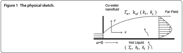
Figure 1 The physical sketch.
narrow slit to the upper surface of the plate, while the lower surface of the plate is heated or cooled by convection from a fluid of temperatureTf. With the assumptions that () the fluid is incompressible and the flow is laminar, () the nanofluid is dilute, () the shape of the metal nanoparticles suspended in the fluid is spherical, and () the homogeneous model developed by Maïgaet al.[] is employed, the velocity and temperature within the momentum and thermal boundary layers, which develop along the surface, can be written as
∂u
∂x +
∂υ
∂y = , ()
u∂u
∂x+υ
∂u
∂y=
μnf
ρnf
∂u
∂y, ()
u∂T
∂x +υ
∂T
∂y =αnf
∂T
∂y, ()
subject to boundary conditions
u= , υ= , –knf
∂T
∂y =hf(x)(Tf–T) aty= , u→, T→T∞, asy→ ∞.
()
Here the Cartesian coordinates system (x,y) is chosen with thex-axis being measured along the plate and they-axis being normal to it, respectively.uandvare the velocity components along thex- andy-axes,Tis the temperature,hf(x) is the heat transfer coef-ficient due toTf;μnf,ρnf,αnf, andknf are, respectively, the viscosity, the density, and the diffusivity and thermal conductivity of the nanofluid, which are given by
μnf =
μf
( –φ)., ρnf = ( –φ)ρf +φρs, αnf =
knf (ρCp)nf
,
(ρCp)nf = ( –φ)(ρCp)f+φ(ρCp)s,
knf
kf
=(ks+ kf) – φ(kf –ks) (ks+ kf) +φ(kf –ks)
,
()
Maxwell-Garnetts model [] with the assumption that the shape of the nanoparticles is restricted to spherical ones.
We now introduce the following similarity variables:
ψ=νf·x/·f(η), η=
νf·x–/·y, θ(η) = T–T∞
Tf–T∞
, ()
whereψ is the stream function defined byu=∂ψ/∂yandv= –∂ψ/∂x, andνf is the kine-matic viscosity of the base fluid.
Substituting Eq. () into Eqs. ()-(), the continuity equation () is automatically satisfied, and the momentum equation () and the energy equation () are reduced to
εf+ff+ f= , ()
ε
Prθ
+fθ= , ()
subject to the boundary conditions
f() = , f() = , θ() = –γ –θ(), f(∞) = , θ(∞) = , () wherePr=νf/αf is the Prandtl number,γ is the reduced heat transfer parameter, andε andεare two constants related to the properties of nanofluids and are given as
ε=
( –φ).[( –φ) +φρ
s/ρf]
, ε=
knf/kf
( –φ) +φ(ρCp)s/(ρCp)f
. ()
The physical quantities of practical interest are the local skin friction coefficientCfxand the local Nusselt numberNux, which are given by
Cfx=
τw
ρfur
, Nux=
xqw
kf(Tw–T∞), () whereτw=μnf(∂u/∂y)y=is the wall shear stress,qw= –knf(∂T/∂y)y=is the wall heat flux, andur= (/)x–/is the reference velocity.
In terms of similarity variables (), we are able to obtain the non-dimensional expres-sions forCfxandNuxvia Eq. () as
CfxRe/x = f()
( –φ)., NuxRex
–/= –knf kf
θ()
θ(), ()
whereRex= (urx)/νf is the local Reynolds number. 3 Analytical solutions
3.1 Asymptotic analysis
Here we check the asymptotic behaviors of the velocity profilef(η) and the temperature profileθ(η) in the limit caseη→ ∞. Due to the boundary conditions (), for considerably largeη, we have
lim
η→∞f
(η)→, lim
Integratingf(η) overηone time, we obtain
lim
η→∞f(η)→λ, ()
whereλis an integral constant. For the physical constraintf≥, it is readily seen that
λ≥.
Forη→ ∞, we supposef(η) andθ(η) can be expressed by
f(η) =λ+F(η), θ(η) =(η), ()
whereF(η) and(η) are negligibly small.
Substituting Eq. () into Eqs. () and () and then linearizing them, we obtain
εF+λF= , ()
ε
Pr
+λ= , ()
which have the explicit solutions
F(η) =Cexp
–λ
ε
η
+C, ()
(η) =Cexp
–λPr
ε
η
, ()
whereC,C, andCare integral constants. Due to Eqs. () and (), it is known that
F== asη→ ∞. ()
With substitution of the boundary condition () into Eq. (), we findC= , which leads to
F(η) =Cexp
–λ
ε
η
. ()
It can be seen from Eqs. () and () thatF(η) and(η) (hencef(η) andθ(η)) decay exponentially asη→ ∞.
3.2 The implicit solution forf(
η
)We multiply Eq. () byf(η) and integrate it fromηto∞, obtaining
εff–
ε f
+ff= . ()
Multiplying Eq. () byf–/and integrating again, we obtain
εf–/f+ f
It is found here that iff(η) is the solution of Eq. (), so isf(η) =Af(Aη), since for any constantA,f(η) always satisfies the boundary conditions (). WhenAvaries, the expres-sions forψandηchange accordingly, anduis precisely the same as that of changing the value of the arbitrary constant velocityUtoU/A. Without loss of generality, we choose
f(∞) = so that the constant in Eq. () is equal to /. Writef =g; we then havef= gg. Therefore Eq. () takes the form
εg=
–g, ()
which has the implicit solution
η=ε
log +g+g
–g
+√arctan
√
g
+g
. ()
By replacinggwithf/, Eq. () can further be written as
η=ε
log +f /+f –f/
+√arctan
√
f/ +f/
. ()
3.3 The explicit solutions forf(
η
) andθ
(η
)Based on the above mentioned asymptotic analysis forf(η) andθ(η) and the homotopy analysis method (HAM), it is assumed that they can be expressed by a set of real functions in the following forms:
f(η) = ∞
k=
fk(η),
θ(η) = ∞
k=
θk(η),
()
wherefk(η) andθk(η) are the high order deformation derivatives and are given by
fk(η) =A¯k+ k+
j=
σkjA¯jkexp(–λjη), ()
θk(η) = k+
j=
ωjkB¯jkexp(–λjη), ()
whereλis a given positive constant, andσkjandωjkare the coefficients defined as
σkj=
, ≤j≤k+ , , other cases, ω
j k=
, ≤j≤k– ,
, other cases. ()
The recursive coefficientsA¯jkandB¯jkfork≥ are determined by
¯
Ak= , ()
¯
¯
Ak=χkσk–A¯k–+Ck, ()
¯
Ak= – f λ
G¯k+C˜k
, ()
¯
Ajk= f
λ(j– )(j– )j
G¯jk–+C˜kj–+B˜kj–+ A˜jk–
, ()
¯
Bk=χkωk–B¯k–+Ck, ()
¯
B
k=χkωk–B¯k–+ λ
PrF¯
k+E˜k
, ()
¯
Bjk=χkωjk–B¯jk–+
λj(j+ )
PrF¯
j– k +E˜
j– k +D˜
j– k
, ()
wheref andθare the HAM auxiliary parameters;Ck,Ck, andCkare integral constants
given by
Ck= –f λ
G¯k+C˜k
– k+
j=
f
λ(j+ )(j+ )
G¯jk+C˜kj+B˜jk+ A˜jk
,
Ck= f λ
G¯k+C˜k
+ k+
j=
f
λj(j+ )
G¯kj+C˜ j k+B˜
j k+ A˜
j k
,
Ck= –
γ + k+
j=
λj+
γ λj(j+ )
PrF¯
j k+E˜
j k+D˜
j k
–
γ+
λ+ γ
λ
PrF¯
k+E˜k
,
()
and
χk=
, k= ,
, k> . ()
Other coefficients appearing in the above recursive formulas are defined as
¯
Ckj= (–λj)σkjA¯jk, E¯jk= (λj)σkjA¯jk, G¯jk= (–λj)σkjA¯jk,
¯
Djk= (–λj)ωjkB¯jk, F¯kj= (λj)ωjkB¯jk,
() and ˜ Aj k= k– n=
max{k–n,j–}
s=max{,j–n–}
¯
Cks––nC¯nj–s,
˜ Bj k= k– n=
max{k–n,j–}
s=max{,j–n–}
¯
Ask––nE¯jn–s,
˜ Cj
k= k–
n=[j–]
¯
˜ Dj
k= k–
n=
max{k–n,j–}
s=max{,j–n–}
¯
Ask––nD¯jn–s,
˜ Ej
k= k–
n=[j–]
¯
A k––nD¯jn,
where [x] gives the greatest integer less than or equal tox. When we setA¯
= ,A¯= –,A¯= ,B¯= ,B¯= –λ/(γ + λ), the purely explicit solu-tions forfk(η) andθk(η) (f(η) andθ(η)) can be determined successively fork= , , , . . . . Note that here the homotopy auxiliary linear operators are selected as
Lf=
∂ ∂η + λ
∂ ∂η + λ
∂
∂η, Lθ= ∂ ∂η +λ
∂
∂η, ()
and the homotopy auxiliary functions are chosen by
f(η) =exp(–λη), θ(η) =exp(–λη). ()
4 Results and discussion
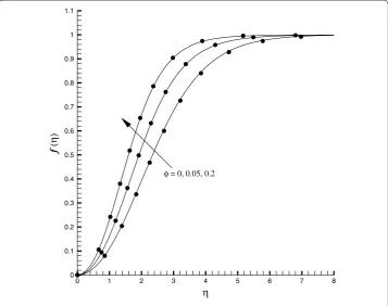
We first examine the reliability and consistency of the explicit solutionf(η) denoted in Eq. (). As shown in Figure , for various values ofφ, our explicit solution agrees well with the implicit one given in () in the whole range ≤η<∞. Further, to check the
Figure 2 Comparison of the implicit solutions (25) with the explicit solutions at 100th order truncations for various values ofφin the case off= –3/2.Circle: the implicit solutions; line: the explicit
Table 1 Computational errors for Errθwithf= –3/2 andθ= –1 in the case ofPr= 1
kth order φ= 20/100,γ= 1 φ= 8/100,γ= 1/2
0 8.18646×10⁻³ 4.04103×10⁻³
30 1.48150×10⁻⁴ 1.44346×10⁻⁵
60 6.73996×10⁻⁵ 4.55130×10⁻⁶
90 3.01452×10⁻⁵ 2.26475×10⁻⁶
120 2.74295×10⁻⁵ 1.37636×10⁻⁶
150 2.31459×10⁻⁵ 9.35413×10⁻⁷
180 6.82566×10⁻⁷
The nanofluid isCu-water.
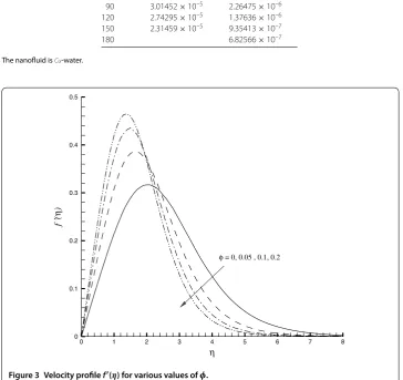
Figure 3 Velocity profilef(η) for various values ofφ.
accuracy of the explicit solutionθ(η), we define the following error estimation function:
Errθ= lim ηs→∞
ηs
ε
Prθ
+fθdη. ()
Substituting various orders of explicit solutionsf(η) andθ(η) into Eq. (), the corre-sponding errors can be obtained, as listed in Table . It is clearly seen from this table that the errors decrease monotonously with the increase of the computational orderkfor both considered cases. The accuracies of those explicit solutions can be further improved when more and more orders of HAM truncations are involved.
The variation of the non-dimensional velocity profilesf(η) withηfor various values of
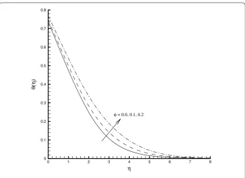
Figure 4 Temperature profilesθ(η) for various values ofφwithPr= 1 andγ= 1.
other hand, we notice that the solid volumetric fraction parameterφplays an important role in the variation off(η); the larger is the value ofφ, the greater is the maximum velocity
f(η). We further notice that the peak velocity of the flow increases withφenlarging, but the critical value ofηcvaries contrarily, it decreases asφincreases. This can be explained by two reasons. One is that the higher concentration nanofluid flow possesses more ki-netic energy than the lower concentration nanofluid or Newtonian fluid flows since they have the same incidence velocities. The other reason is that, unlike Newtonian fluid flows that are usually subject to a solid boundary, the nanofluid flows past a geometry are often restricted by a slip boundary, which is of help to reduce the flow drag near the resting wall. We then consider the variation of the non-dimensional temperature profilesθ(η) with
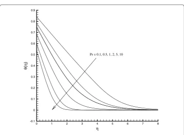
ηfor various values ofφin the case ofPr= andγ = . As illustrated in Figure ,θ(η) decreases continuously asηevolves for any prescribed value ofφ. On the other hand,θ(η) enhances smoothly withφincreasing. This shows that the heat transfer characteristics of the considered fluid can be gradually improved as appropriate nanoparticles are continu-ally added to it. We also notice that the reduced heat transfer parameterγ has an obvious effect onθ(η). As shown in Figure , the temperature profileθ(η) increases consecutively asγ enlarges for allη. This changing trend becomes more evident for small values ofγ. We further notice that, asγ tends to ,θ(η) approaches as well. In this limiting case, there is no heat transfer by convection through the wall at all. Asγ tends to∞,θ(η) ap-proaches . In this limiting case, the wall temperature is equal to the temperature of the fluid under the wall. Following that, we discuss the effect of the Prandtl number Pron the variation ofθ(η). As shown in Figure ,θ(η) diminishes consecutively asPrincreases. This trend is very similar to the case of the Newtonian fluid flow, but the variation range forθ(η) is apparently smaller as compared with that of the Newtonian fluid flow. When
Figure 5 Temperature profilesθ(η) for different values ofγwithφ= 0.1 andPr= 1.
Figure 7 Variation of the reduced local skin friction coefficientCfxwithφ.
The local skin friction coefficientCfxand the local Nusselt numberNuxare practically important in various applications regarding the flow and heat transfer in the boundary layer region. We therefore discuss them successively. As shown in Figure ,Cfxenlarges almost linearly asφevolves from to .. Using the explicit solution forf(η), one readily gives the explicit expression forCfxRe/x , due to Eq. (),
CfxRe/x = ( –φ).
+∞
k= k+
j=
(λj)σkjA¯jk. ()
Figure gives the variation of the reduced Nusselt numberNuxRe–/x withφforPr= and
γ = /. It is found thatNuxRe–/x increases gradually withφincreasing, but its changing range is slower than that ofCfxRe/x . Though it is not shown in this paper, it is found that
γ has little effect on the variation ofNuxRe–/x , it is almost unchanged for all ranges <
γ <∞. Similarly, we are able to give the explicit expression forNuxRe–/x in the following form:
NuxRex–/= –
knf kf
+∞
k= k+
j=
(–λj)ωjkB¯jk
+∞
k= k+
j=
¯
Bjk
. ()
The boundary layer thicknesses are of physical importance for this problem, defined by
δf/x= ηfδ/Re/x , δθ/x= ηδθ/Re/x , () whereδf is the thickness of the velocity boundary layer andδθis the thickness of the
Figure 8 Variation of the reduced Nusselt numberNuxwithφforγ= 1/10 andPr= 1.
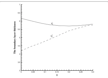
boundary layers are located at the pointsηδf andηδθwithf(ηδf) andθ(ηδθ) having the same value of .. The variations of the boundary layer thicknessesηδ
f andηθδwithφare
plot-ted in Figure . It is seen from the figure that theηδ
f increases continuously asφenlarges from to .; beyond this value, its value decreases asφevolves.ηδθexhibits a totally dif-ferent trend, its values increase gradually asφincreases from to .. But its increasing rate gradually descends asφevolves, particularly, whenφ≥., its effect onηδθbecomes dramatically small. It is worth mentioning that the homogeneous model is only valid for small values ofφ,i.e.≤φ≤.. Whenφis considerably large, the nanofluid shows the characteristics of non-Newtonian fluids and this model cannot predict the behaviors of the nanofluid accurately.
5 Conclusions
In this paper, the laminar jet flow and heat transfer of a copper-water nanofluid over a rest-ing wall has been examined in detail. By means of the homogeneous model, the original Navier-Stokes equations describing these jet flows have been reduced to a set of differen-tial equations. An analytical solution for the velocity distribution has been obtained. The explicit solutions for both the velocity and the temperature distributions have been given by means of the HAM technique. The effects of the volumetric fraction parameterφand the dimensionless heat transfer coefficientγ on the velocity and temperature profiles, as well as on the reduced local skin friction coefficient and the reduced Nusselt number have been investigated. Some novel results and findings of this study have been presented:
. An implicitly analytical solution for the velocity distribution is given, which has not been reported before.
Figure 9 Variation of the boundary layer thicknesses ofηf
δandηθδwithφforγ= 1/10 andPr= 1.
. Purely explicit solutions with high precision for both the velocity and the temperature distributions are obtained.
. The volumetric fraction parameterφhas an important effect on the velocity and temperature distribution. The maximum velocity increases asφenlarges. The temperature profiles increase asφevolves, too. This means that the addition of nanoparticles into pure fluids is of help to reduce the flow drag near the wall and to improve the heat transfer capability of the base fluids.
. The dimensionless heat transfer parameterγ plays a key role on the variation of the temperature profiles. The temperature profiles enhances asγ increases.
Competing interests
The authors declare that they have no competing interests.
Authors’ contributions
All authors contributed equally to the writing of this paper. All authors read and approved the final manuscript.
Author details
1State Key Lab of Ocean Engineering, School of Naval Architecture, Ocean and Civil Engineering, Shanghai Jiao Tong
University, Shanghai, 200240, China. 2Department of Computer Science and Engineering, Shanghai Jiao Tong University, Shanghai, 200240, China.
Acknowledgements
We extend our sincere appreciations to the Program for New Century Excellent Talents in University (Grant No. NCET-12-0347), and to the Program of Innovative Fundings for Youth of the State Key Laboratory of Ocean Engineering (Shanghai Jiao Tong University) (Grant No. GKZD010059-17) for their financial supports.
Received: 13 December 2013 Accepted: 15 April 2014 Published: 1 September 2014
References
1. Glauert, MB: The wall jet. J. Fluid Mech.16, 625-643 (1956)
5. Cohen, J, Amitay, M, Bayly, BJ: Laminar-turbulent transition of wall jet flows subjected to blowing and suction. Phys. Fluids A4, 283-289 (1992)
6. Xu, H, Liao, SJ, Wu, GX: A family of new solutions on the wall jet. Eur. J. Mech. B, Fluids27, 322-334 (2008) 7. Magyari, E, Keller, B, Pop, I: Heat transfer characteristics of a boundary-layer flow driven by a power-law shear over a
semi-infinite flat plate. Int. J. Heat Mass Transf.47, 31-34 (2004)
8. Cossali, GE: Similarity solutions of energy and momentum boundary layer equations for a power-law shear driven flow over a semi-infinite flat plate. Eur. J. Mech. B, Fluids25, 18-32 (2006)
9. Fan, T, Xu, H: New branches with algebraical behaviour for thermal boundary-layer flow over a permeable sheet. Commun. Nonlinear Sci. Numer. Simul.18, 1162-1174 (2013)
10. Choi, SUS: Enhancing thermal conductivity of fluids with nanoparticle. In: The Proceedings of the 1995 ASME International Mechanical Engineering Congress and Exposition, ASME, FED 231/ MD66, San Francisco, USA, November 12-17, pp. 99-105 (1995)
11. Maïga, SEB, Palm, SJ, Nguyen, CT, Roy, G, Galanis, N: Heat transfer enhancement by using nanofluids in forced convection flows. Int. J. Heat Fluid Flow26(4), 530-546 (2005)
12. Xuan, YM, Roetzel, W: Conceptions for heat transfer correlation of nanofluids. Int. J. Heat Mass Transf.43(19), 3701-3707 (2000)
13. Buongiorno, J: Convective transport in nanofluids. J. Heat Transf.128(3), 240-250 (2006)
14. Buongiorno, J, Hu, W: Nanofluid coolants for advanced nuclear power plants. In: Proceedings of ICAPP ’05, Paper no. 5705, Seoul, May 15-19 (2005)
15. Trisaksri, V, Wongwises, S: Critical review of heat transfer characteristics of nanofluids. Renew. Sustain. Energy Rev.11, 512-523 (2007)
16. Wang, XQ, Mujumdar, AS: Heat transfer characteristics of nanofluids: a review. Int. J. Therm. Sci.46, 1-19 (2007) 17. Eastman, JA, Phillpot, SR, Choi, SUS, Keblinski, P: Thermal transport in nanofluids. Annu. Rev. Mater. Res.34, 219-246
(2004)
18. Kakac, S, Pramaumjaroenkij, A: Review of convective heat transfer enhancement with nanofluids. Int. J. Heat Mass Transf.52, 3187-3196 (2009)
19. Bachok, N, Ishak, A, Pop, I: Flow and heat transfer over a rotating porous disk in a nanofluid. Physica B406, 1767-1772 (2011)
20. Rohni, AM, Ahmad, S, Pop, I: Flow and heat transfer over an unsteady shrinking sheet with suction in nanofluids. Int. J. Heat Mass Transf.55, 1888-1895 (2012)
21. Yacob, NA, Ishak, A, Pop, I: Falkner-Skan problem for a static or moving wedge in nanofluids. Int. J. Therm. Sci.50, 133-139 (2011)
22. Vajravelu, K, Prasad, KV, Lee, J, Lee, C, Pop, I, Vab Gorder, RA: Convective heat transfer in the flow of viscous Ag-water and Cu-water nanofluids over a stretching surface. Int. J. Therm. Sci.50, 843-851 (2011)
23. Aziz, A: A similarity solution for laminar thermal boundary layer over a flat plate with a convective surface boundary condition. Commun. Nonlinear Sci. Numer. Simul.14, 1064-1068 (2009)
24. Ishak, A: Similarity solutions for flow and heat transfer over a permeable surface with convective boundary condition. Appl. Math. Comput.217, 837-842 (2010)
25. Aziz, A, Khan, WA: Natural convective boundary layer flow of a nanofluid past a convectively heated vertical plate. Int. J. Therm. Sci.52, 83-90 (2012)
26. Makinde, OD, Aziz, A: MHD mixed convection from a vertical plate embedded in a porous medium with a convective boundary condition. Int. J. Therm. Sci.49, 1813-1820 (2010)
27. Hayat, T, Iqbal, Z, Qasim, M, Obaidat, S: Steady flow of an Eyring Powell fluid over a moving surface with convective boundary conditions. Int. J. Heat Mass Transf.55, 1817-1822 (2012)
28. Brinkman, HC: The viscosity of concentrated suspensions and solutions. J. Chem. Phys.20, 571-581 (1952) 29. Xuan, Y, Li, Q: Investigation on convective heat transfer and flow features of nanofluids. J. Heat Transf.125, 151-155
(2003)
doi:10.1186/1687-2770-2014-163
Cite this article as:Raees et al.:Explicit solutions of wall jet flow subject to a convective boundary condition.