American Journal of Remote Sensing
2013; 1(2) : 21-32Published online April 2, 2013 (http:// www.sciencepublishinggroup.com/j/ajrs) doi: 10.11648/j.ajrs.20130102.12
An efficient hybrid classification system for high resolution
remote sensor data
Roopesh Tamma
1, T. Ch. Malleswara Rao
2, G. Jaisankar
1 1Dept of Geo Engineering, Andhra University, Visakhapatnam, India 2
School of Electronics, Sreenidhi Institute of Technology, Hyderabad, India
Email address:
[email protected] (R. Tamma), [email protected] (T. Ch. Malleswara Rao), [email protected](G. Jaisankar)
To cite this article:
Roopesh Tamma, T. Ch. Malleswara Rao, G. Jaisankar. An Efficient Hybrid Classification System for High Resolution Remote Sensor Data, American Journal of Remote Sensing. Vol. 1, No. 2, 2013, pp. 21-32. doi: 10.11648/j.ajrs.20130102.12
Abstract:
The classification of aerial and satellite remote sensing data has become a challenging problem due to the recent ad-vances in remote sensor technology that led to higher spatial and spectral resolutions. This research paper presents novel sensor independent algorithms and techniques for dealing with the challenges of classification of high volume remote sensor data. A fast unsupervised band reduction method is proposed to lower the dimensionality of the input image. The band reduced image is then split into two mutually disjoint pure and mixed pixel subsets by a pixel segregator built using extended mathematical morphology techniques. A novel hierarchical spectral-spatial support vector machine based classifier that adaptively includes the usage of ex-pensive spatial information based on the pixel categorization is proposed. The final thematic map is obtained after merging the classification results of the two subsets and fixed spatial neighborhood homogenization. The accuracy, efficiency and flexibility of the developed system are demonstrated by evaluating the classification results using several hyperspectral and multispectral data sets. The obtained results demonstrate that the proposed method performs significantly better than conventional classifiers while alleviating the computational complexity involved in generating spatial information.Keywords:
Morphological Profile Operators, Spectral And Spatial Classification, Vector Ordered Statistics, Support Vector Machine (SVM), Hyperspectral, Multispectral1. Introduction
Conventional pixel by pixel classifiers of remote-sensing data are based on signal modeling where statistical signal-based classification algorithms are applied on spectral infor-mation of each pixel vector and the pixel is assigned to the class that has the most similar statistical spectral characteristics. High spatial resolution data contains a lot of contextual infor-mation that can be employed to achieve higher discrimination of various spectrally similar classes. Many traditional classifi-ers can be enhanced by inclusion of spatial and contextual in-formation. Consequently, joint spatial and spectral classifiers have been developed to analyze the remote sensing data better [1, 2]. Majority of the combined spatial and spectral metho-dologies presented act on a single-band image [3, 4]. Linear extension of these grayscale techniques to multi- or hyperspec-tral data will not be meaningful due to the problem of ordering
accu-22 Roopesh Tamma et al.: An efficient hybrid classification system for high resolution remote sensor data
racy while keeping the computation cost within an acceptable range.
Conventional statistical supervised classification methods are also hindered by limited availability of ground truth data and their inefficiency in handling high dimensional data. Over the last decade many techniques have been proposed to ad-dress the complexity and accuracy issues [8, 9, 10]. However, the available techniques are still inadequate for better utility of high resolution data. To deal with the statistical estimation ineptness in the presence of unfavorable ratio between availa-ble training samples to the features, several alternatives have been proposed to reduce the variance of the estimate for li-mited training samples [11, 12], but these improvements still suffer from the risk of over fitting the few available training samples and lead to a poor approximation of statistics. This stresses the need for a data model that has low sensitivity to the number of training samples. SVMs are shown to have ca-pabilities for handling problems related to classification of RS data with robustness to dimensionality, good generalization ability, and a non-linear decision function. Support Vector Ma-chine (SVM) is a new and very promising classification tech-nique developed by Vapnik and his group at AT&T Bell Labs [13]. Recently, researchers are focusing more on the study of SVM due to its useful applications in a number of areas, such as pattern recognition, multimedia, image processing and bio-informatics [14, 15, 16].
In the context of all the aforementioned issues, the purpose of this research is to develop a set of new techniques to obtain effective, efficient and improved classification of high resolu-tion data collected from satellite and airborne platforms. The accuracy, efficiency and flexibility of the developed methods and software are demonstrated by evaluating the classification results using several hyperspectral and multispectral data sets with a wide variety of spatial and spectral resolutions and en-compassing diverse contexts such as urban, semi-urban and agricultural scenes. The results obtained when compared with the results of conventional spectral-only and spectral-spatial classifiers indicate that higher accuracies can be achieved with the use of these techniques and the proposed methods also alleviate the computational complexity involved by adaptive application of expensive spatial information.
This paper is organized in to five sections. Section II gives an overview of the proposed algorithms. Experimental data and setup are described in section III, and results are discussed in section IV. Section V concludes the paper.
2. Proposed Method
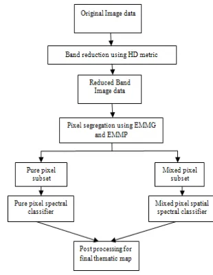
The flowchart of the proposed hierarchical hybrid classifica-tion scheme is show in Fig. 1. The input image data set is first subjected to an unsupervised dimensionality reduction algo-rithm to eliminate redundant bands. The band reduced image is then segregated into pure and mixed pixel subsets using
ex-tended mathematical morphological operators. Pixels identi-fied as pure are classiidenti-fied using only the spectral features, whereas classification of pixels marked as mixed employs both spectral and spatial information. The mixed pixels are then homogenized by application of an adjacency majority marker algorithm to eliminate presence of any detached classified pix-els in the thematic map. The input to the classifier is an n band multi- or hyper spectral image and the output will be a themat-ic classified map assigning each pixel of the input a unique class label. As shown, the classification system consists of the following four main phases:
• Band Reduction
• Pure and mixed pixel segregation
• Classification using SVMs of mixed and pure pixel subsets
o Pure pixels classified using spectral
fea-ture vectors and a simple Radial basis function (RBF) kernel.
o Mixed pixels classified using a hybrid
spectral and spectral feature vector and a composite hybrid RBF kernel.
• Post-classification homogenization and merging. Each of these phases is described in detail below.
Figure 1. General architecture of the proposed classification system.
2.1. Band Reduction
American Journal of Remote Sensing 2013, 1(2) : 21-32 23
band selection methods for efficiency, a method based on Hamming distance (HD) metric is proposed. HD metric, in addition to being an unsupervised technique has the huge ben-efit of computationally very fast as it does not involve any higher order calculations and can be applied with the need for any object information. HD between two image band vectors
Bi = {pi1, pi2… pin} and Bj = {pj1, pj2… pjn}, where n is the total
number of pixels and pix represents pixel value at offset x in
band i, is given by the following expression.
HD(Bi, Bj) = ∑ (1)
The basic idea is that if two adjacent bands do not differ greatly then the underlying spectral-spatial property can be characterized by only one band. In general, adjacent bands that differ significantly should be retained, while similar adjacent bands can be reduced. The proposed algorithm for band reduc-tion is presented below. In the algorithm the final Hamming distance threshold ϵ chosen will be arrived at by iteratively adjusting the threshold, starting with zero and incrementing, till the desired band count is achieved. The final band count chosen depends on the accuracy requirements and computa-tional resources available to the user. Table 1 presents the pro-posed band reduction algorithm. The final band count chosen depends on the accuracy requirements and computational re-sources available to the user.
Table 1. Band reduction algorithm using Hamming distance metric.
Procedure BandReduction(Iband1...bandn, η, Є) Inputs:
Orignial Image: I Number of bands: η
Hamming distance threshold: Є Outputs:
Reduced band image Ibr Begin
i = 0, Ibr = {Ø}, j = i+1, while (j < η)
forall pixel vectors p in Bandi, and pj in Bandj Hnet = H(Bi, Bj),
if (Hnet < Є) then Ibr = Ibr {Bj}, j = j+1, Else
i = j, j = i+1, Endif EndWhile Return Ibr End
2.2. Pure and Mixed Pixel Segregation
The current methods available for multi or hyper spectral
data analysis are inherently either pure pixel techniques, where each pixel is considered to be spectrally homogenous, or mixed pixel techniques where each pixel is treated as essential-ly spectralessential-ly heterogeneous. Many a times, the image set is often a combination of heterogeneous and homogenous pixels, where many sites in a scene are pure materials but many others are mixture of multiple elements. As part of this research work, it is proposed and shown that segregating the input multi or hyper spectral image data set into pure pixels and mixed pixels as a pre-classification step will help improve the accuracy and computational expense during the classification phase.
The segregation algorithm proposed is based on the ob-served properties of edges. Edges in any image formation model correspond to changes in discontinuities of physical properties. Generally, edges indicate overlap of two or more homogenous areas and thus, majority of the mixed pixels should lie on the edges. Features on edges have sharp bounda-ries. Because of the limited spatial resolution of remotely sensed images pixels on edges will contain a mixture of spec-tral responses from different features. Though edge detection in gray valued images is well studied, the task is less well de-fined in multi- or hyperspectral images. Techniques based on manifold learning [7], clustering and multivariate statistical approaches [17] were proposed to extract edges. Many of these techniques though perform satisfactorily on multispectral im-ages, are not well suited for higher dimensional hyperspectral images. Also, these conventional algorithms like Sobel, Prewitt and Laplacian of Gaussian operator [18] are not a good fit for edge detection in images with multiple object boundaries, sha-dows and noise.
Filters based on mathematical morphology (MM) enable much more accurate definition of pixel neighborhoods and spatial structures in image scene than the conventional fixed closed neighborhoods at a much lower computational cost [19, 20]. The proposed pure and mixed pixel segregation algorithm uses extended mathematical morphological (EMM) operators.
dimen-24 Roopesh Tamma et al.: An efficient hybrid classification system for high resolution remote sensor data
sions as a set of pixel vectors {x1, ..., xn} and a distance metric
d(xi, xj) to evaluate the ordering distance between two pixel
vectors xi and xj, for a set of pixel vectors within a flat
struc-turing element B, dB(x) defines the cumulative distance
be-tween one particular pixel vector xi and all the other pixel
vec-tors in the spatial neighborhood defined by B.
dB(x) = Σ(dB(x, xj)) ∀xj∈ B (2)
dB(x) can then be used to define the supremum and infimum
given a set of vectors. For a given set of vectors X, dB(x) is
computed for every element in the set and the infimum is cho-sen as that xi for which dB(xi) is the mimimum and similarly,
the supremum is defined as the xi for which dB(xi) is maximum
of that set. The choice of the distance metric is an important factor in obtaining an effective ordering relation and here a L1 norm was used.
Following the vector and EMM notation described in the previous chapter, the extended mathematical morphological gradient (EMMG) of an image can be obtained by computing the image difference between the dilated and eroded images. Computing the EMMG and applying a suitable threshold θ yields the edge contours. Pixels lying on these contours are most likely candidates to be marked as mixed. Additionally, further refinement of this likely-mixed pixel subset using ex-tended mathematical morphological profiles (EMMP) is fur-ther done to identify strictly mixed pixels to achieve even greater dimensionality reduction. EMMP construction was first proposed in [6] for segmentation of high resolution images.
The algorithm for pixel segregation is given in Table 2. The output of the algorithm will be two mutually disjoint subset image of the originally image, one subset containing all the pure pixels and the other subset made of all the pixels marked as mixed, and these two subsets are used as an input to the classification phase. In the algorithm listed below, (p ∘/● B)i denotes a geodesic dilation/erosion repeated i iterations. To determine the change between EMMPs in successive iterations, HD operator is used as the metric. The iteration count parame-ter k for the algorithm theoretically needs to be the value at which morphological idempotency is reached and, empirically it was found that a value of 5 to 7 provides good results.
Table 2. Algorithm for categorizing a pixel as pure or mixed pixel.
Procedure: PixelVectorType(I, B, θ, k, refine) Inputs:
InputImage: I, Sructuring Element: B, EMMG threshold: θ, Max # of iterations: k, Additional refinement flag: refine
Outputs:
Pixel Type: Mixed or pure for a pixel vector Begin:
# Compute EMMG IG = EMMG(I)
For each pixel p(x, y) in IG
If d(p(x, y)) > θ then Pixeltype = Mixed Elseif
Pixeltype = Pure If refine == FALSE then Return,
For each pixel p(x, y) in IG marked as mixed # Compute extended opening MP
For i=0 to k EMPio(p)= (p o B)i
# Compute extended closing MP For i=0 to k
EMPi●(p) = (p ● B)i
# Compute the derivatives of EMMP For i=1 to k
DEMPio = H(EMPio(p), EMPi-1o(p)) DEMPi● = H(EMPi●(p), EMPi-1●(p)) If ∨ DEMPio(p) > ∨ DEMPi●(p) then Pixeltype = Pure
Elseif
Pixeltype = Mixed Endif
Return (PixelType) End
2.3. Classification using Hybrid SVM
SVMs with higher generalization capability, robustness to dimensionality, lower effort for model selection during learn-ing phase and optimality of solution have proven to be more effective than the conventional parametric or non-parametric classifiers [24]. Due to all the benefits offered by SVM, in this work a hybrid classifier based on SVM method is proposed. SVM classifier design consists of choosing the appropriate feature vectors, model selection and selection of a multi-class classifier architecture.
nonli-American Journal of Remote Sensing
nearities into the SVM problem and the performance of the resulting SVM will often hinge on the appropriate choice of the kernel. Though there are many kernels available in ture, the RBF kernel was chosen for this work. This kernel, unlike the linear kernel, can handle problems where the rel tion between class labels and attributes in not linear
kernel also has the additional benefit of having fewer hyper parameters and hence a lower model complexity
two tunable parameters: the penalty parameter radius parameter. A multi-class is then built using one
one approach as the training time is much smaller compared to other approaches [26].
2.4. Post-classification Processing
The previous classification step produces two different cla sification maps, one for the pure-pixel sub-image and one for the mixed-pixel sub-image, with each pixel in the map a signed a unique class label. The post-classification processing contains merging the two disjoint classification maps to create the full image classification map, and applying contextual i formation regularization over the local neighborhood of all the mixed pixels.
Merging of the classification maps is a straight forward m thod of performing a union of the tow classification maps. The thematic map obtained from the merging operation is further refined by the application of a fixed neighborhood majority vote spatial regularization procedure for each of the mixed pixels. The area for regularization is defined by an 8
neighborhood. For each mixed pixel in the classification map, the label of the pixel is replaced by the majority vote i.e. the label with highest frequency in the chosen neighborhood area. The majority vote procedure might have to be repeated for a few iterations until stability is reached. Application of regul rization reduces noise in the classification map and more h mogenous regions in the final thematic map and elimi
“salt-and-pepper” effect. The regularized classification map will be the final thematic map.
3. Data and Experimental Setup
For evaluating the performance of techniques developed in this work a set of hyperspectral and multispectral images from different sensors with varying spatial and spectral resolutions and covering a diverse variety of contexts and different spe tral and spatial resolutions are used. Details of the data sets are listed in Table 3. Performance of the proposed algorithms was evaluated both qualitatively and quantitatively against results obtained by conventional methods. The classification system was implemented in C and run on a Linux x86 platforms. A widely used SVM library libsvm [29] was used to perform basic SVM related tasks.
American Journal of Remote Sensing 2013, 1(2) : 21-32
nearities into the SVM problem and the performance of the resulting SVM will often hinge on the appropriate choice of the kernel. Though there are many kernels available in
litera-kernel was chosen for this work. This litera-kernel, unlike the linear kernel, can handle problems where the rela-tion between class labels and attributes in not linear [25]. RBF kernel also has the additional benefit of having fewer
hyper-meters and hence a lower model complexity and has only two tunable parameters: the penalty parameter C and λ the class is then built using one-against-one approach as the training time is much smaller compared to
The previous classification step produces two different clas-image and one for image, with each pixel in the map
as-classification processing contains merging the two disjoint classification maps to create the full image classification map, and applying contextual in-formation regularization over the local neighborhood of all the
tion maps is a straight forward me-thod of performing a union of the tow classification maps. The thematic map obtained from the merging operation is further refined by the application of a fixed neighborhood majority or each of the mixed pixels. The area for regularization is defined by an 8-way fixed neighborhood. For each mixed pixel in the classification map, the label of the pixel is replaced by the majority vote i.e. the neighborhood area. The majority vote procedure might have to be repeated for a few iterations until stability is reached. Application of regula-rization reduces noise in the classification map and more ho-mogenous regions in the final thematic map and eliminates any
pepper” effect. The regularized classification map
. Data and Experimental Setup
the performance of techniques developed in and multispectral images from ifferent sensors with varying spatial and spectral resolutions and different spec-are used. Details of the data sets spec-are . Performance of the proposed algorithms was aluated both qualitatively and quantitatively against results The classification system was implemented in C and run on a Linux x86 platforms. A was used to perform
Table 3. Details of data sets chosen for experimental evaluation
Data set Name Sensor Type Spectral Range # of Band s Image Size in pixels Indian Pines AVI-RISa air-borne
10 nm
covering the wa-velength range from 0.4 to 2.5 µm
220 145x145
Universi-ty of Pavia ROSISb air-borne
2.9 nm covering range from 400 to 970 nm
102 1096x10 96
Ananta-pur
IRSc
-1B LISSd-I
0.46 –
0.86µm 4
512 x
512
Ujjain
IRS-P6 LISS-IV
0.52
-0.86 µm 3
512 x
512
a Airborne Visible/Infrared Imaging Spectrometer
b Reflective Optics System Imaging Spectrometer
c Indian Remote Sensing Satellite.
d Linear Imaging Self Scanner.
Figure 2. Indian Pines 220 band AVIRIS hyerspectral data set (a) False color composite image. (b) Training ground truth mask.
ground truth file. (d) Legend for ground truth masks with test and train sample counts shown in parenthesis as (test_sample_count,
25
Details of data sets chosen for experimental evaluation.
Image Size in pixels
Location Resolu-tion Groun d Truth classes Refer Fig-ure No. 145x145 Indian Pines site in Northwes-tern Indiana, USA [27]
20m 16 2
1096x10 Pavia, northern Italy [28]
1.3m 9 3
512 x
Anantapur area, Andhra Pradesh, India
72.5m 15 4
512 x
Ujjain area, Madhya Pradesh, India
5.8m 9 5
Airborne Visible/Infrared Imaging Spectrometer.
Reflective Optics System Imaging Spectrometer.
Indian Pines 220 band AVIRIS hyerspectral data set (AVIRIS, 1992). (a) False color composite image. (b) Training ground truth mask. (c) Test ground truth file. (d) Legend for ground truth masks with test and train sample
26 Roopesh Tamma et al.: An efficient hybrid classification system for high resolution remote sensor dat
Figure 3. University of Pavia 103 band ROSIS sensor data set
(a) False color composite image. (b) Test ground truth mask. (c) Training ground truth mask. (d) Legend for the ground truth mask with test and train sample counts given in parenthesis as (test_sample_count,
train_sample_count).
Figure 4. IRS-1B LISS-I 4 band Anantapur data set. (a) False color composite image. (b) Test ground truth mask. (c) Training ground truth mask. (d) Legend for the ground truth mask with test and train sample counts given in par sis as (test_sample_count, train_sample_count).
Figure 5. IRS-P6 LISS-IV 3 band Ujjain data set. (a) False color composite image. (b) Test ground truth mask. (c) Training ground truth mask. (d) Legend
.: An efficient hybrid classification system for high resolution remote sensor dat
University of Pavia 103 band ROSIS sensor data set (Pavia, 2002). composite image. (b) Test ground truth mask. (c) Training ground truth mask. (d) Legend for the ground truth mask with test and train
test_sample_count,
data set. (a) False color composite truth mask. (c) Training ground truth mask. (d) Legend for the ground truth mask with test and train sample counts given in
parenthe-IV 3 band Ujjain data set. (a) False color composite ground truth mask. (d) Legend
for the ground truth with test and train sample counts shown in parenthesis as (test_sample_count, train_sample_coun
4. Experimental Results
The proposed algorithms and techniques have been ev luated for accuracy and performance with the data sets sented in the previous section. The results of the experiments are discussed in this section.
4.1. Band Reduction Algorithm Performance
The proposed band reduction method was applied on the I dian Pines and University of Pavia data set to evaluate the pe formance and utility. Classification accuracy and computatio al complexity are the metrics used for the purpose of eval tion. The metrics are obtained on a pixel wise SVM based spectral classifier. Results of band reduction experiments on the Indian Pines data set are tabulated in Table
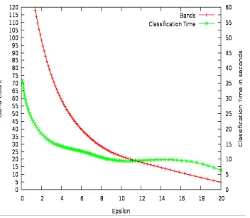
bands are eliminated, the accuracy gradually increases while the classification time drops steeply. This increase in accuracy as the dimensionality decreases can be explained by the Hughes phenomenon. Reduction of the bands should help filter out redundant features that add to the confusion in the decision process. Though the table does not present the memory r quirements, it can be deduced that the memory requirements also drop proportional to the number of bands eliminated. Fig 6 shows the plots that indicate the rate of band elimination and accuracy for changing values of the
the algorithm is tightly depended on the choice of effective
Table 4. Band reduction performance for Indian Pines data set
Epsilon ϵϵϵϵ Band Count Avg Acc
0.1 183 73.40%
0.4 168 74.2%
0.8 124 76.55%
1.0 109 79.15%
2.0 83 81.89%
3.0 62 82.19%
4.0 51 81.76%
5.0 46 82.34%
6.0 37 82.06%
7.0 33 53.14%
8.0 24 80.06%
9.0 22 79.16%
10.0 21 78.80%
12.0 19 76.34%
15.0 12 70.64%
20.0 5 53.10%
.: An efficient hybrid classification system for high resolution remote sensor data
for the ground truth with test and train sample counts shown in parenthesis as test_sample_count, train_sample_count).
4. Experimental Results
The proposed algorithms and techniques have been eva-luated for accuracy and performance with the data sets pre-. The results of the experiments
rithm Performance
The proposed band reduction method was applied on the In-dian Pines and University of Pavia data set to evaluate the per-formance and utility. Classification accuracy and computation-al complexity are the metrics used for the purpose of evcomputation-alua- evalua-tion. The metrics are obtained on a pixel wise SVM based spectral classifier. Results of band reduction experiments on the Indian Pines data set are tabulated in Table 4. As more bands are eliminated, the accuracy gradually increases while tion time drops steeply. This increase in accuracy dimensionality decreases can be explained by the Hughes phenomenon. Reduction of the bands should help filter out redundant features that add to the confusion in the decision le does not present the memory re-quirements, it can be deduced that the memory requirements also drop proportional to the number of bands eliminated. Fig. shows the plots that indicate the rate of band elimination and accuracy for changing values of the threshold ϵ. The success of the algorithm is tightly depended on the choice of effective ϵ.
Band reduction performance for Indian Pines data set
Overall Acc Classification Time (in secs)
71.92% 36.01
72.99% 27.10
72.45% 21.33
72.81% 17.43
73.94% 14.16
74.58% 13.21
74.17% 11.13
75.07% 11.11
74.41% 11.12
62.13% 11.01
70.81% 10.19
71.11% 7.17
70.93% 9.57
68.17% 8.48
62.82% 13.49
American Journal of Remote Sensing
Figure 6. The effect of ϵ on band count and the relation between band count
and accuracy for the Indian Pines data set.
From the curves it can be deduced that the classification pe formance drops steeply at ϵ = 8.0. After this point, the loss of features due to band elimination negatively affects the classif cation accuracy even though the classification time is greatly reduced. Fig. 7 plots the band count and classification time against ϵ. The observed unusual increase in the classification time even with lower band count is probably due to the add tional overhead involved in cross-validation phase of SVM parameter tuning. The graphs demonstrate that the best trade off between computation time and accuracy for
occurs at ϵ =8.0.
Figure 7. The effect of ϵ on band count and how the changing band count effects the classification time for the Indian Pines data set
Results of band reduction on the University of Pavia data set are tabulated in Table 5. Figure 8 gives the rate of band elim nation and accuracy for changing values of the threshold Fig. 9 plots the band count and classification time against Similar to the results of the Indian Pines data set, the accuracy monotonically increases to a point after which it steeply drops as the number of bands eliminated increases. After the infle tion point, a gradual decrease of accuracy can be observed as the classification becomes less reliable due to loss of inform tion. The proposed method is economical and efficient as it relies on only self contained components without the need for
American Journal of Remote Sensing 2013, 1(2) : 21-32
on band count and the relation between band count
the classification per-= 8.0. After this point, the loss of
gatively affects the classifi-cation accuracy even though the classificlassifi-cation time is greatly
plots the band count and classification time . The observed unusual increase in the classification bly due to the addi-validation phase of SVM parameter tuning. The graphs demonstrate that the best
trade-computation time and accuracy for this band set
on band count and how the changing band count effects the classification time for the Indian Pines data set.
Results of band reduction on the University of Pavia data set gives the rate of band elimi-or changing values of the threshold ϵ and plots the band count and classification time against ϵ. Similar to the results of the Indian Pines data set, the accuracy monotonically increases to a point after which it steeply drops s eliminated increases. After the inflec-tion point, a gradual decrease of accuracy can be observed as the classification becomes less reliable due to loss of informa-tion. The proposed method is economical and efficient as it
omponents without the need for
supervised validation, expensive optimization or exhaustive search based band selection processes. The experimental r sults demonstrate that significant gains can be obtained even by application of coarse band reduction with
of accuracy.
Table 5. Band reduction performance evaluation for the University of Pavia data set.
Epsilon ϵϵϵϵ Band Count Avg Acc
0.1 103 80.59%
0.2 93 80.69%
0.4 70 80.98%
0.8 43 82.55%
1.0 37 84.71%
2.0 19 83.37%
3.0 13 79.69%
4.0 9 80.00%
5.0 7 76.38%
6.0 5 71.99%
10.0 3 69.52%
Figure 8. The effect of ϵ on band count and the relation between band count and accuracy for the University of Pavia data set.
Figure 9. The effect of ϵ on band count and how the changing band count effects the classification time for the University of Pavia data set.
27
expensive optimization or exhaustive band selection processes. The experimental re-sults demonstrate that significant gains can be obtained even by application of coarse band reduction without noticeable loss
Band reduction performance evaluation for the University of Pavia
Overall Acc Classification Time (in secs)
74.14% 181
74.34% 156
74.78% 124
79.57% 93
81.20% 84
82.29% 68
79.29% 62
78.46% 60
78.29% 54
70.88% 59
68.86% 73
on band count and the relation between band count and accuracy for the University of Pavia data set.
28 Roopesh Tamma et al.: An efficient hybrid classification system for high resolution remote sensor data
4.2. Classification Results
The performance of the proposed classifier system is eva-luated against two other conventional classifiers, the Maxi-mum Likelihood (ML) classifier and Extraction and Classifica-tion of Homogenous Objects (ECHO) classifier [1] and the original pixel-wise SVM spectral classifier. ML classifier is well known and powerful statistical probabilistic classifier used for supervised classification. ML classification is done by using pixel-wise spectral signatures only. ECHO classifier is widely used in remote sensing community for joint spectral and spatial classification that relies on partitioning the image into statistically homogenous regions and then classifies each region as a single object. ECHO and ML classifications were performed using the widely used academic hyper- or multis-pectral image processing software MultiSpec [30]. Comparing results against the results produced by popular software pro-vides for not only a complete but also a fair and bias free in-vestigation.
Wherever possible, the same band reduced image is used as input for all the various classifiers. The accuracy is measured using the overall accuracy, average accuracy and Kappa coef-ficient performance measures described in a previous section. A small set of the available ground truth data was chosen as training data. Accuracies are calculated by using the trained model on the test ground truth data. Thematic maps are created for the entire data sets.
Indian Pines Data Set
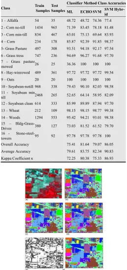
The 220-band Indian Pines data set was first reduced to a 46 band image using ϵ=5.0. The feature vector for spectral classi-fication was made up of the reflectance values of each of the band. For the hybrid SVM, applying pixel segregation with θ=12.0 yielded a mixed pixel map with 51.48% of the pixels being marked as mixed. SVM parameters (C, λ) were tuned to (32, 0.5) using cross validation. Table 6 gives the class-specific and overall accuracies for all the classifiers applied on the In-dian Pines data set. The classification maps and the mixed pix-el maps are shown in Fig. 10. From the results we can see that for majority of the classes the ECHO classifier out performs both pixel–wise ML and SVM classification. For classes that are already homogenous, the SVM classifier performs better than the ML and at least as good as the ECHO classifier. This bolsters the idea that incorporating spatial information greatly enhances the classification accuracy of heterogeneous regions with a higher proportion of mixed pixels. The best global and class accuracies are obtained when applying joint spectral and spatial information using a hybrid SVM. The hybrid SVM sig-nificantly out performs both the SVM and ECHO classifier and this confirms the effectiveness of using EMMP as feature vector. From visual inspection it can be observed that misclas-sification occurs mostly between classes that are essentially close variants of each other (such as the corn and soya va-riants).
Table 6. Classification results for the Indian Pines data set.
Class Train
Samples Test Samples
Classifier Method Class Accuracies ML ECHO SVM SVM
Hybr-id
1 – Alfalfa 54 35 48.72 48.72 74.36 77.4
2 - Corn no-till 1434 965 71.39 83.45 78.18 81.48
3 - Corn min-till 834 467 63.01 75.13 69.64 83.93
4 – Corn 234 178 85.87 92.39 91.85 98.37
5- Grass Pasture 497 308 93.51 94.18 92.17 97.54
6 - Grass tress 747 236 94.69 96.27 91.68 97.70
7 - Grass pasture
mowed 26 25 36.36 100 100 100
8 - Hay-winrowed 489 361 97.72 97.72 97.72 99.54
9 – Oats 20 20 100 100 100 100
10 - Soyabean-notill 968 338 79.43 90.10 82.03 98.58 11 - Soyabean min
till 2468 265 52.65 64.14 58.95 82.09
12 - Soyabean clean 614 333 85.99 89.89 87.94 97.70
13 – Wheat 212 109 98.15 98.15 98.77 99.38
14 – Woods 1294 553 95.42 94.21 93.01 98.38
15 –
Bldg-Grass-Drives 380 127 73.03 81.52 61.52 79.70
16 -
Stone-steel-towers 95 92 97.78 97.78 97.78 100
Overall Accuracy 75.41 81.64 79.07 86.05
Average Accuracy 79.61 83.75 82.34 90.83
Kappa Coefficient κ 72.25 80.38 75.33 86.93
Figure 10. Indian Pines data set (a) False color composite. (b) MLC classifi-cation map. (c) ECHO classifier classificlassifi-cation map. (d) SVM classificlassifi-cation map. (e) Mixed pixel map (dark pixels indicate mixed pixels). (f) SVM-hybrid classification map.
University of Pavia Data Set
American Journal of Remote Sensing 2013, 1(2) : 21-32 29
using band reduction algorithm with ϵ set to 1.0. SVM parame-ters (C, λ) were tuned to (32.0, 2.0) using cross-validation. Table 7 reports the class and global accuracies for the Univer-sity of Pavia data set. The classification thematic maps are shown in Fig. 11. Again, it is apparent from the summarized results that the classification accuracies reported by spatio-spectral methods exceed spatio-spectral only methods significantly. Also the accuracy gain by the hybrid SVM compared to the ECHO classifier is higher than the Indian Pines data set. One probable reason for this is that this scene contains proportion-ally more straight lines with different orientations than the Indian pines scene. This demonstrates that the spatial features using EMMP provides a final classification output that is cohe-rent in both spectral and spatial terms for a complex real-world analysis scenario.
Table 7. Classification results for the University of Pavia data set.
Class Train
Samples Test Sam-ples
Classifier Method Class Accuracies ML ECHO SVM SVM Hybrid
1 - Roof 412 3834 95.75 96.22 95.64 97.60
2 - Street 124 416 71.39 83.45 94.48 81.48
3 - Paths 175 175 63.01 75.13 97.71 83.93
4 - Grass 1928 313 85.87 92.39 99.53 98.37
5- Trees 405 212 93.51 94.18 79.16 97.54
6 - Water 1224 271 94.69 96.27 97.22 97.70
7 - Shadow 97 45 36.36 100 100 100
Overall Accuracy 75.41 81.64 79.17 86.05
Average Accuracy 79.61 83.75 85.97 90.83
Kappa Coefficient
κ 72.25 80.38 75.33 86.93
Figure 11. University of Pavia data set. (a) False color composite. (b) MLC classification map. (c) ECHO classification map. (d) SVM classification map. (e) Mixed pixel map (dark pixels indicate mixed pixels). (f) SVM-hybrid classi-fication map.
Anatapur Data Set
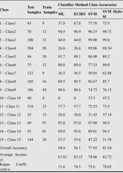
For this data set no band reduction was done as the image has only four bands. With θ = 2, 59% of the pixels are identi-fied as mixed. The higher proportion of mixed pixels is ex-plained by the coarser resolution of the sensor and the hetero-gonous composition of the land area. Using cross validation the SVM parameters (C, λ) were tuned to (2048.0, 2.0). Table 8 presents the classification results and the classification the-matic maps are shown in Fig. 12. SVM hybrid outperforms all the other classifiers. The conventional classifiers perform bad-ly on some classes, this can probabbad-ly be explained by the fact that training regions chosen are are heterogeneous spanning across boundaries, and the possibility of incorrectly labeled training samples. ML and ECHO classifiers could not classify class 10 as the scarcity of training samples leads to covariance matrix inversion failure. SVM and SVM-hybrid classifiers were able to handle this situation and this demonstrates the robustness of the SVM based classifiers in the presence of a small training set. SVM based classifiers, unlike conventional classifiers also performed significantly better even with mixed training samples.
Table 8. Classification results for Anantaupur data set.
Class Test
Samples Train Samples
Classifier Method Class Accuracies ML ECHO SVM SVM
Hybr-id
1 – Class1 45 9 37.8 67.8 77.78 75.9
2 – Class2 78 12 94.9 94.9 96.15 98.71
3 – Class3 100 12 44.0 44.0 99.00 99.0
4 – Class4 384 20 26.6 26.6 89.06 88.54
5 – Class5 84 30 85.7 88.1 86.90 89.2
6 – Class6 75 12 80.0 80.0 77.33 80.0
7 – Class7 132 9 36.5 36.5 59.85 62.88
8 – Class8 105 16 89.5 89.5 86.67 85.7
9 – Class9 186 44 80.6 80.6 74.73 76.13
10 – Class 10 40 4 0 0 37.5 47.5
11 –Class 11 318 25 37.7 37.7 72.33 73.9
12 – Class 12 35 12 38.0 38.0 31.43 37.14
13 – Class 13 99 97 97.0 97.0 97.98 98.9
14 – Class 14 91 81 89.0 95.6 89.01 94.5
15 – Class 15 144 20 53.5 55.6 47.22 51.38
Overall Accuracy 54.4 56.1 77.92 81.54
Average
Accura-cy 67.81 83.15 74.86 82.72
Kappa
30 Roopesh Tamma et al.: An efficient hybrid classification system for high resolution remote sensor dat
Figure 12. Anantapur data set. (a) False color composite. (b) MLC classific tion map. (c) ECHO classification map. (d) SVM classification map. (e) Mixed pixel map. (f) SVM-hybrid classification map.
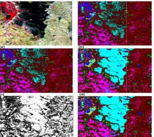
Ujjain Data Set
This data set is made up of only three channels and
band reduction procedure was applied to this data set. With θ = 2.5, 36.4% of the pixels are marked as mixed and the SVM parameters (C, λ) were tuned to (32, 0.5). Table
classification results with various classifiers. Fig
classification thematic maps. Comparing the results it can be observed that SVM did only marginally better t
and both methods have similar problems of misclassification of built-up land and agricultural area. SVM performs slightly worse than the MLC for certain agricultural classes, though on average the SVM performs better. This is probably due to th small deviation of the spectral data from normal distributions. The use of spatial information and homogenization of solitary pixels results in much better results for the ECHO classifier and SVM hybrid classifier.
Table 9. Classification results for Ujjain data set.
Class Test
Samples Train Samples
Classifier Method Class Accuracies
ML ECHO
1 – Class1 648 238 93.7 94.7
2 – Class2 948 266 87.6 87.7
3 – Class3 384 180 90.9 99.2
4 – Class4 435 100 68.0 77.7
5 – Class5 415 187 96.9 96.9
6 - Class6 3371 432 91.3 91.3
7 – Class7 1263 330 91.7 91.7
8 – Class8 1820 416 73.0 73.0
9 – Class9 400 143 84.3 84.3
Overall Accuracy 86.5 87.2
Average Accuar-cy
86.3 86.9
Kappa Coefficient κ
83.7 84.5
.: An efficient hybrid classification system for high resolution remote sensor dat
Anantapur data set. (a) False color composite. (b) MLC classifica-classification map. (e) Mixed
This data set is made up of only three channels and hence no band reduction procedure was applied to this data set. With θ s mixed and the SVM parameters (C, λ) were tuned to (32, 0.5). Table 9 shows the classification results with various classifiers. Fig. 13 shows the classification thematic maps. Comparing the results it can be observed that SVM did only marginally better than the MLC and both methods have similar problems of misclassification up land and agricultural area. SVM performs slightly worse than the MLC for certain agricultural classes, though on average the SVM performs better. This is probably due to the small deviation of the spectral data from normal distributions. The use of spatial information and homogenization of solitary pixels results in much better results for the ECHO classifier
Ujjain data set.
Classifier Method Class Accuracies ECHO SVM SVM
Hybr-id
95.04 95.12
89.76 89.76
92.97 99.61
41.72 81.33
96.90 96.90
98.96 99.82
88.04 92.01
75.34 75.34
84.51 86.11
88.29 91.13
88.41 90.67
86.11 89.28
Figure 13. Ujjain data set. (a) False color composite. (b) MLC classification map. (c) ECHO classification map. (d) SVM
pixel map. (f) SVM-hybrid classification map.
The results demonstrate that the SVM
more suitable and efficient for the classification of data sets with high dimensions as well as multispectral images. As was observed from the results of all the classifiers, it is quite appa ent that the incorporating spatial inform
homogenization using some form of inter
measures results in visually and qualitatively better classific tion maps. The hybrid SVM, by use of EMMG includes the boundary information in the yields classification maps with accurate borders. Lowering of the dimensionality by a fast and efficient band reduction method resulted in huge computatio al expense savings. Also, in particular, as majority of the i ages are composed of homogenous regions, limiting the appl cation of spatial information only for pixels identified as mixed decreased the computational needs of the hybrid class fication. On average, the proposed methodology resulted in 5 10% increase in classification accuracies without incurring any significant computational overhead.
5. Conclusions
This paper presented new algorithms and a system for sor independent effective and efficient classification of hyper or multispectral images. The proposed algorithms include a fast unsupervised dimensionality reduction
computationally economical algorithm for segregating pixels in the image into mixed and pure pixel categories and an ada tive hybrid classification method that selectively applies the spatial information along with spectral information.
tive of this work was the need for incorporating spatial and spectral information in multi- or hyperspectral image classif cation process without incurring a huge overhead in terms of computational performance. The proposed methodology su ceeds in satisfying this need by taking advantage of the fact that tradeoff between accuracy and computation cost is ma imized by limiting the extraction and use of spatial features
.: An efficient hybrid classification system for high resolution remote sensor data
Ujjain data set. (a) False color composite. (b) MLC classification map. (c) ECHO classification map. (d) SVM classification map. (e) Mixed
hybrid classification map.
The results demonstrate that the SVM method is technically more suitable and efficient for the classification of data sets with high dimensions as well as multispectral images. As was observed from the results of all the classifiers, it is quite appar-ent that the incorporating spatial information and performing homogenization using some form of inter-pixel dependency measures results in visually and qualitatively better classifica-tion maps. The hybrid SVM, by use of EMMG includes the boundary information in the yields classification maps with accurate borders. Lowering of the dimensionality by a fast and efficient band reduction method resulted in huge computation-al expense savings. Also, in particular, as majority of the im-ages are composed of homogenous regions, limiting the appli-patial information only for pixels identified as mixed decreased the computational needs of the hybrid classi-fication. On average, the proposed methodology resulted in 5-10% increase in classification accuracies without incurring any
nal overhead.
This paper presented new algorithms and a system for sen-effective and efficient classification of hyper-or multispectral images. The proposed alghyper-orithms include a fast unsupervised dimensionality reduction scheme, an elegant computationally economical algorithm for segregating pixels in the image into mixed and pure pixel categories and an adap-tive hybrid classification method that selecadap-tively applies the spatial information along with spectral information. The objec-tive of this work was the need for incorporating spatial and
or hyperspectral image classifi-cation process without incurring a huge overhead in terms of computational performance. The proposed methodology
American Journal of Remote Sensing 2013, 1(2) : 21-32 31
only for the subset of pixels which mostly benefit by the use of this information in the classification process. Evaluation of the proposed techniques against existing methods has demonstrat-ed that, on average, an increase of 5-10% overall accuracy has been observed with less than 40% computational cost increase. Following the direction of current research for effective han-dling of high spatial and spectral resolution data, some of the issues that remain open and conducive for further research are identified. Application of a fast search based scheme to further optimize the proposed band reduction scheme might result in improved performance. As many of the tasks in the classifica-tion scheme lend themselves to be parallelizable both within and across modules, attempt at splitting and concurrent han-dling of these actions will result in reduction of overall classi-fication time.
References
[1] Kettig, R. L., and Landgrebe D. (1976). Classification of mul-tispectral image data by extraction and classification of homo-genous objects, IEEE Transactions on Geoscience Electronics, Vol. 14, No. 1, pp. 19-26.
[2] Landgrebe D.A. (1980). The development of a spectral-spatial classifier for earth observational data. Pattern Recognition, Vol. 12, pp. 165-175.
[3] Dobson, M. C., Pierce, L., Kellndorfer, J., and Ulbay, F. (1997). Use of SAR image texture in terrain classification. IEEE Trans. On Geosci. and Remote Sens., Vol. 3, No. 1, pp. 1180-1184. [4] de Jong, S. M., Hornstra, T.J., and Mass, H. (2001). An
inte-grated spatial and spectral approach to the classification of Me-diterranean land cover types: the SSC method. JAG, Vol. 3, No. 2, pp. 176-183.
[5] Tarabalka, Y., Bendiktsson, J. A., and Chanussot, J. (2010). SVM and MRF-based method for accurate classification of hyperspectral images. IEEE Trans. Geosci. Remote Sens., Vol 7, No. 4, pp. 736-740.
[6] Benediktsson, J. A., Plamson, J. A., and Sveinsson, J. (2005). Classification of hyperspectral data from urban areas based on extended morphological profiles. IEEE Transactions on Geos-cience and Remote Sensing, Vol. 43, No. 3, pp. 480–491. [7] Zhou, Y., Wu, B., Li, D., and Li, R. (2009). Edge detection on
hyperspectral imagery via manifold techniques. IEEE Workshop on Hyperspectral Image and Signal Processing, WHISPERS’09, Grenoble, France.
[8] Goel, P. K., Prasher, S. O., and Patel, R. M, Landry, J. A., Bon-nell, R. B., and Viau, A. A. (2003). Classification of hyperspec-tral data by decision trees and artificial neural networks to iden-tify weed stress and nitrogen status of corn, Comput. Electron. Agricult., Vol. 39, pp. 67–93.
[9] Landgrebe., D. (2003). Signal Theory Methods in Multispectral Remote Sensing, John Wiley & Sons, Inc., 2003.
[10] Camp-Valls, G., Bruzzone, L. (2005). Kernel-based methods for
hyperspectral image classification, IEEE Transactions on Geos-cience and Remote Sensing, vol. 43. No. 6, pp. 1351-1362. [11] Hoffbeck, J. P. and Landgrebe, D. A (1996), Covariance matrix
estimation and classification with limited training data, IEEE Transactions Pattern Anal. Machine Intelligence, Vol. 8, pp. 763-767.
[12] Tajudin, S., Landgrebe, D. A. (1999). Covariance estimation with limited training samples, IEEE Transactions on Geoscience Remote Sensing, Vol. 37, No. 4, pp. 2113-2118.
[13] Vapnik, V. N (1998). Statistical learning theory. Wiley, New York.
[14] Joachims, T. (1998). Making large scale SVM learning practical. In B. Scholkopf, C. Burges, & A. Smola (Eds.), Advances in Kernel methods-support vector learning. MIT Press, New York. [15] Cristianini, N., and Shawe-Taylor, J. (2000). An introduction to
support vector machines and other Kernel-based learning me-thods. Cambridge University Press, Cambridge.
[16] Kecman, V. (2001). Learning and soft computing — support vector machines, neural networks, fuzzy logic systems. MIT Press, Cambridge.
[17] Verszkov, S., and Paclik, P. (2006). Edge detection in hyper-spectral imaging – multivariate statistical approaches. Structural, Syntactic and Statistical Pattern Recognition, 4109, 551–559. [18] Huertas, A., Medioni, G. (1986). Detection of intensity changes
with subpixel accuracy using Laplacian-Gaussian masks, IEEE Transactions on Pattern Analysis and Machine Intelligence, Vol. 8, No. 5, pp. 651-664.
[19] Serra, J. (1982). Image Analysis and Mathematical Morphology, vols. 1 and 2. Academic Press, San Diego.
[20] Epifanio, I., Soille, P. (2003). Segmentation of natural land-scapes using morphological texture features, Geoscience and Remote Sensing Symposium, IEEE-IGARSS Proceedings, Vol. 1, pp. 445-457.
[21] Louverdis, G., Andreadis, I., Tsalides, P. (2002). New fuzzy model for morphological color image processing, Vision, Image and Signal Processing, IEEE Proceedings, vol. 149, no. 3, pp. 129-139.
[22] Astolaa, J., Haavisto, P., & Neuvo, Y. (1990). Vector Median Filter. Proceedings of the IEEE, Vol. 78, No. 4, pp. 679-689. [23] Evans, A., and Liu, X. (2006). A morphological gradient
ap-proach to color edge detection. IEEE Transactions on Image Processing, Vol. 15, No. 6, pp. 1454–1463.
[24] Melgani, P., Bruzzone, L. (2004). Classification of hyperspec-tral remote sensing images with support vector machines, IEEE Transactions on Geoscience and Remote Sensing, vol. 42, no. 8, pp. 1778-1790.
32 Roopesh Tamma et al.: An efficient hybrid classification system for high resolution remote sensor data
[26] Hsu, C., and Lin, C. (2002). A comparison of methods for multi-class support vector machines, IEEE Transactions on Neural Networks, Vol. 13, No. 2, pp. 415-425.
[27] AVIRIS (1992). AVIRIS NW Indiana’s Indian Pines 1992 data set. ftp://ftp.ecn.purdue.edu/biehl/Multispec/92AV3C.lan(data set) and ftp://ftp.ecn.purdue.edu/biehl/Multispec/ ThyFiles.zip (ground truth). Accessed 24 Jan, 2011.
[28] Pavia University (2000). University of Pavia data set. www.ehu.es/uploads/e/ee/PaviaU.mat (data set) and www.ehu.es/uploads/5/50/PaviaU_gt.mat (ground truth).
Ac-cessed 24 Jan, 2011.
[29] Chang, C., and Lin, C. (2001). LIBSVM: a library for support vector machines. Software available at http://www.csie. ntu.edu.tw/~cjlin/libsvm. Accessed 24 Jan 2011.