Learning Module Networks

Learning Module Networks

Eran Segal [email protected]

Computer Science Department Stanford University

Stanford, CA 94305-9010, USA

Dana Pe’er [email protected]

Genetics Department Harvard Medical School Boston, MA 02115, USA

Aviv Regev [email protected]

Bauer Center for Genomic Research Harvard University

Cambridge, MA 02138, USA

Daphne Koller [email protected]

Computer Science Department Stanford University

Stanford, CA 94305-9010, USA

Nir Friedman [email protected]

Computer Science & Engineering Hebrew University

Jerusalem, 91904, Israel

Editor: Tommi Jaakkola

Abstract

Methods for learning Bayesian networks can discover dependency structure between observed variables. Although these methods are useful in many applications, they run into computational and statistical problems in domains that involve a large number of variables. In this paper,1 we consider a solution that is applicable when many variables have similar behavior. We introduce a new class of models, module networks, that explicitly partition the variables into modules, so that the variables in each module share the same parents in the network and the same conditional probability distribution. We define the semantics of module networks, and describe an algorithm that learns the modules’ composition and their dependency structure from data. Evaluation on real data in the domains of gene expression and the stock market shows that module networks generalize better than Bayesian networks, and that the learned module network structure reveals regularities that are obscured in learned Bayesian networks.

1. Introduction

Over the last decade, there has been much research on the problem of learning Bayesian networks from data (Heckerman, 1998), and successfully applying it both to density estimation, and to dis-covering dependency structures among variables. Many real-world domains, however, are very complex, involving thousands of relevant variables. Examples include modeling the dependencies among expression levels (a rough indicator of activity) of all the genes in a cell (Friedman et al., 2000a; Lander, 1999) or among changes in stock prices. Unfortunately, in complex domains, the amount of data is rarely enough to robustly learn a model of the underlying distribution. In the gene expression domain, a typical data set describes thousands of variables, but at most a few hundred instances. In such situations, statistical noise is likely to lead to spurious dependencies, resulting in models that significantly overfit the data.

Moreover, if our goal is structure discovery, such domains pose additional challenges. First, due to the small number of instances, we are unlikely to have much confidence in the learned structure (Pe’er et al., 2001). Second, a Bayesian network structure over thousands of variables is typically highly unstructured, and therefore very hard to interpret.

In this paper, we propose an approach to address these issues. We start by observing that, in many large domains, the variables can be partitioned into sets so that, to a first approximation, the variables within each set have a similar set of dependencies and therefore exhibit a similar behavior. For example, many genes in a cell are organized into modules, in which sets of genes required for the same biological function or response are co-regulated by the same inputs in order to coordinate their joint activity. As another example, when reasoning about thousands of NASDAQ stocks, entire sectors of stocks often respond together to sector-influencing factors (e.g., oil stocks tend to respond similarly to a war in Iraq).

We define a new representation called a module network, which explicitly partitions the variables into modules. Each module represents a set of variables that have the same statistical behavior, i.e., they share the same set of parents and local probabilistic model. By enforcing this constraint on the learned network, we significantly reduce the complexity of our model space as well as the number of parameters. These reductions lead to more robust estimation and better generalization on unseen data. Moreover, even if a modular structure exists in the domain, it can be obscured by a general Bayesian network learning algorithm which does not have an explicit representation for modules. By making the modular structure explicit, the module network representation provides insight about the domain that are often be obscured by the intricate details of a large Bayesian network structure. A module network can be viewed simply as a Bayesian network in which variables in the same module share parents and parameters. Indeed, probabilistic models with shared parameters are common in a variety of applications, and are also used in other general representation languages, such as dynamic Bayesian networks (Dean and Kanazawa, 1989), object-oriented Bayesian

Net-works (Koller and Pfeffer, 1997), and probabilistic relational models (Koller and Pfeffer, 1998;

Friedman et al., 1999a). (See Section 8 for further discussion of the relationship between module networks and these formalisms.) In most cases, the shared structure is imposed by the designer of the model, using prior knowledge about the domain. A key contribution of this paper is the design of a learning algorithm that directly searches for and finds sets of variables with similar behavior, which are then defined to be a module.

INTL MSFT

MOT

AMAT

DELL HPQ

CPD 4

P(INTL) MSFT

CPD 6 CPD 6 CPD 3

CPD 5 CPD 1

CPD 2

INTL MSFT

MOT

DELL

Module 3 Module 2

Module 1

CPD 3 CPD 2 CPD 1

AMAT

HPQ

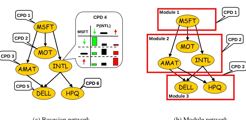
(a) Bayesian network (b) Module network

Figure 1: (a) A simple Bayesian network over stock price variables; the stock price of Intel (INTL) is annotated with a visualization of its CPD, described as a different multinomial dis-tribution for each value of its influencing stock price Microsoft (MSFT). (b) A simple module network; the boxes illustrate modules, where stock price variables share CPDs and parameters. Note that in a module network, variables in the same module have the same CPDs but may have different descendants.

to modules and the probabilistic model for each module. We evaluate the performance of our al-gorithm on two real data sets, in the domains of gene expression and the stock market. Our results show that our learned module network generalizes to unseen test data much better than a Bayesian network. They also illustrate the ability of the learned module network to reveal high-level structure that provides important insights.

2. The Module Network Framework

We start with an example that introduces the main idea of module networks and then provide a formal definition. For concreteness, consider a simple toy example of modeling changes in stock prices. The Bayesian network of Figure 1(a) describes dependencies between different stocks. In this network, each random variable corresponds to the change in price of a single stock. For illus-tration purposes, we assume that these random variables take one of three values: ‘down’, ‘same’ or ‘up’, denoting the change during a particular trading day. In our example, the stock price of Intel (INTL) depends on that of Microsoft (MSFT). The conditional probability distribution (CPD) shown in the figure indicates that the behavior of Intel’s stock is similar to that of Microsoft. That is, if Microsoft’s stock goes up, there is a high probability that Intel’s stock will also go up and vice versa. Overall, the Bayesian network specifies a CPD for each stock price as a stochastic function of its parents. Thus, in our example, the network specifies a separate behavior for each stock.

in-fluences the stock price of all of the major chip manufacturers — Intel (INTL), Applied Materials (AMAT), and Motorola (MOT). In turn, the stock price of computer manufacturers Dell (DELL) and Hewlett Packard (HPQ), are influenced by the stock prices of their chip suppliers — Intel and Applied Materials. An examination of the CPDs might also reveal that, to a first approximation, the stock price of all chip making companies depends on that of Microsoft and in much the same way. Similarly, the stock price of computer manufacturers that buy their chips from Intel and Applied Materials depends on these chip manufacturers’ stock and in much the same way.

To model this type of situation, we might divide stock price variables into groups, which we call modules, and require that variables in the same module have the same probabilistic model; that is, all variables in the module have the same set of parents and the same CPD. Our example contains three modules: one containing only Microsoft, a second containing chip manufacturers Intel, Applied Materials, and Motorola, and a third containing computer manufacturers Dell and HP (see Figure 1(b)). In this model, we need only specify three CPDs, one for each module, since all the variables in each module share the same CPD. By comparison, six different CPDs are required for a Bayesian network representation. This notion of a module is the key idea underlying the module network formalism.

We now provide a formal definition of a module network. Throughout this paper, we assume that we are given a domain of random variables

X

={X1, . . . ,Xn}. We use Val(Xi) to denote the

domain of values of the variable Xi.

As described above, a module represents a set of variables that share the same set of parents and the same CPD. As a notation, we represent each module by a formal variable that we use as a placeholder for the variables in the module. A module set

C

is a set of such formal variables M1, . . . ,MK. As all the variables in a module share the same CPD, they must have the same domain

of values. We represent by Val(Mj) the set of possible values of the formal variable of the j’th

module.

A module network relative to

C

consists of two components. The first defines a template prob-abilistic model for each module in

C

; all of the variables assigned to the module will share this probabilistic model.

Definition 1 A module network template

T

= (

S

,θ)for

C

defines, for each module Mj∈

C

:

• a set of parents PaMj⊂

X

;

• a conditional probability distribution template P(Mj |PaMj) which specifies a distribution

over Val(Mj)for each assignment in Val(PaMj).

We use

S

to denote the dependency structure encoded by{PaMj : Mj ∈

C

} andθto denote the

parameters required for the CPD templates{P(Mj|PaMj) : Mj∈

C

}.

In our example, we have three modules M1, M2, and M3, with PaM1 = /0, PaM2 ={MSFT}, and PaM3 ={AMAT,INTL}.

The second component is a module assignment function that assigns each variable Xi ∈

X

to

one of the K modules, M1, . . . ,MK. Clearly, we can only assign a variable to a module that has the

same domain.

Definition 2 A module assignment function for

C

is a function

A

:

X

→ {1, . . . ,K} such that

In our example, we have that

A

(MSFT) =1,

A

(MOT) =2,

A

(INTL) =2, and so on.

A module network defines a probabilistic model by using the formal random variables Mjand

their associated CPDs as templates that encode the behavior of all of the variables assigned to that module. Specifically, we define the semantics of a module network by “unrolling” a Bayesian net-work where all of the variables assigned to module Mjshare the parents and conditional probability

template assigned to Mjin

T

. For this unrolling process to produce a well-defined distribution, the

resulting network must be acyclic. Acyclicity can be guaranteed by the following simple condition on the module network:

Definition 3 Let

M

be a triple(

C

,

T

,

A

), where

C

is a module set,

T

is a module network template for

C

, and

A

is a module assignment function for

C

.

M

defines a directed module graph

G

_M as follows:

• the nodes in

G

M correspond to the modules in

C

;

•

G

_M contains an edge Mj→Mkif and only if there is a variable X∈

X

so that

A

(X) = j and

X∈PaMk.

We say that

M

is a module network if the module graph

G

M is acyclic.

For example, for the module network of Figure 1(b), the module graph has the structure M1 → M2→M3.

We can now define the semantics of a module network:

Definition 4 A module network

M

= (

C

,

T

,

A

)defines a ground Bayesian network

B

M over

X

as

follows: For each variable Xi∈

X

, where

A

(Xi) = j, we define the parents of Xiin

B

M to be PaMj,

and its conditional probability distribution to be P(Mj|PaMj), as specified in

T

. The distribution

associated with

M

is the one represented by the Bayesian network

B

M.

Returning to our example, the Bayesian network of Figure 1(a) is the ground Bayesian network of the module network of Figure 1(b).

Using the acyclicity of the module graph, we can now show that the semantics for a module network is well-defined.

Proposition 5 The graph

G

M is acyclic if and only if the dependency graph of

B

M is acyclic.

Proof: The proof follows from the direct correspondence between edges in the module graph and edges in the ground Bayesian network. Consider some edge Xi→Xj in

B

M. By definition of the

module graph, we must have an edge MA(Xi) →MA(Xj) in the module graph. Thus, any cyclic path in

B

M corresponds directly to a cyclic path in the module graph, proving one direction of the

theorem. The proof in the other direction is slightly more subtle. Assume that there exists a cyclic path p= (M1 →M2. . .Ml →M1) in the module graph. By definition of the module graph, if Mi→Mi+1there is a variable Xiwith

A

(Xi) =Mithat is a parent of Xi+1, for each i=1, . . . ,l−1.

By construction, it follows that there is an arc Xi →Xi+1 in

B

M. Similarly, there is a variable

Xl with

A

(Xl) =Ml that is a parent of M1. And so, we conclude that

B

ModNet contains a cycle

X1→X2→. . .

X

l →X1, proving the other direction of the theorem

As we can see, a module network provides a succinct representation of the ground Bayesian network. In a realistic version of our stock example, we might have several thousand stocks. A Bayesian network in this domain needs to represent thousands of CPDs. On the other hand, a module network can often represent a good approximation of the domain using a model with only few dozen CPDs.

3. Data Likelihood and Bayesian Scoring

We now turn to the task of learning module networks from data. Recall that a module network is specified by a set of modules

C

, an assignment function

A

of nodes to modules, the parent structure

S

specified in

T

, and the parametersθfor the local probability distributions P(Mj |PaMj). We assume in this paper that the set of modules

C

is given, and omit reference to it from now on. We note that, in the models we consider in this paper, we do not associate properties with specific modules and thus only the number of modules is of relevance to us. However, in other settings (e.g., in cases with different types of random variables) we may wish to distinguish between different module types. Such distinctions can be made within the module network framework through more elaborate prior probability functions that take the module type into account.

One can consider several learning tasks for module networks, depending on which of the re-maining aspects of the module network specification are known. In this paper, we focus on the most general task of learning the network structure and the assignment function, as well as a Bayesian posterior over the network parameters. The other tasks are special cases that can be derived as a by-product of our algorithm.

Thus, we are given a training set

D

={x[1], . . . ,x[M]}, consisting of M instances drawn indepen-dently from an unknown distribution P(

X

). Our primary goal is to learn a module network structure and assignment function for this distribution. We take a score-based approach to this learning task. In this section, we define a scoring function that measures how well each candidate model fits the observed data. We adopt the Bayesian paradigm and derive a Bayesian scoring function similar to the Bayesian score for Bayesian networks (Cooper and Herskovits, 1992; Heckerman et al., 1995). In the next section, we consider the algorithmic problem of finding a high scoring model.

3.1 Likelihood Function

We begin by examining the data likelihood function

L(

M

:

D

) =P(

D

|

M

) =

M

∏

m=1

P(x[m]|

T

,

A

).

This function plays a key role both in the parameter estimation task and in the definition of the structure score.

As the semantics of a module network is defined via the ground Bayesian network, we have that, in the case of complete data, the likelihood decomposes into a product of local likelihood functions, one for each variable. In our setting, however, we have the additional property that the variables in a module share the same local probabilistic model. Hence, we can aggregate these local likelihoods, obtaining a decomposition according to modules.

More precisely, let Xj={X ∈

X

|

A

(X) = j}, and let θMj|Pa_{M j} be the parameters associated

Instance 3 Module 3 Module 2 Module 1 AMAT θθθθ θθθθ θθθθ DELL HPQ INTL MOT MSFT Instance 1 Instance 2 + MSFT) (AMAT, S + MSFT) (MOT, S MSFT) (INTL, S = MSFT) , (M S (MSFT) S ) (M S = + INTL) AMAT, (DELL, S + INTL) AMAT, (HPQ, S = INTL) AMAT, , (M S

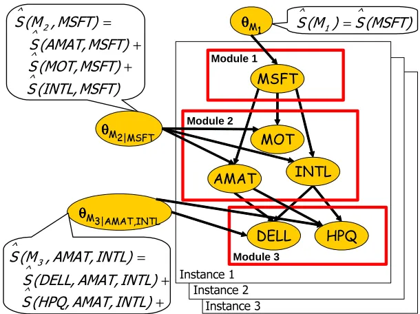
Figure 2: Shown is a plate model for three instances of the module network example of Figure 1(b). The CPD template of each module is connected to all variables assigned to that module (e.g. θ_{M2|MSFT is connected to AMAT, MOT, and INTL). The sufficient statistics of} each CPD template are the sum of the sufficient statistics of each variable assigned to the module and the module parents.

module likelihoods, each of which can be calculated independently and depends only on the values

of Xj and PaMj, and on the parametersθMj|Pa_{M j}:

L(

M

:

D

)

=

K

∏

j=1

"

M

∏

m=1X

∏

i∈Xj

P(xi[m]|paMj[m],θMj|Pa_{M j}) #

=

K

∏

j=1

Lj(PaMj,X j_,θ

Mj|Pa_{M j} :

D

). (1)

If we are learning conditional probability distributions from the exponential family (e.g., discrete distribution, Gaussian distributions, and many others), then the local likelihood functions can be reformulated in terms of sufficient statistics of the data. The sufficient statistics summarize the relevant aspects of the data. Their use here is similar to that in Bayesian networks (Heckerman, 1998), with one key difference. In a module network, all of the variables in the same module share the same parameters. Thus, we pool all of the data from the variables in Xj, and calculate our statistics based on this pooled data. More precisely, let Sj(Mj,PaMj) be a sufficient statistic function for the CPD P(Mj|PaMj). Then the value of the statistic on the data set

D

is

ˆ

Sj= M

∑

m=1X

∑

i∈Xj

For example, in the case of networks that use only multinomial table CPDs, we have one suffi-cient statistic function for each joint assignment x∈Val(Mj),u∈Val(PaMj), which is

η{Xi[m] =x,paMj[m] =u},

the indicator function that takes the value 1 if the event (Xi[m] =x,PaMj[m] =u) holds, and 0 otherwise. The statistic on the data is

ˆ

Sj[x,u] = M

∑

m=1X

∑

i∈Xj

η{Xi[m] =x,PaMj[m] =u}.

Given these sufficient statistics, the formula for the module likelihood function is:

Lj(PaMj,X j_,θ

Mj|Pa_{M j} :

D

) =

∏

x,u∈Val(Mj,Pa_{M j})

θSˆj[x,u]

x|u .

This term is precisely the one we would use in the likelihood of Bayesian networks with multinomial table CPDs. The only difference is that the vector of sufficient statistics for a local likelihood term is pooled over all the variables in the corresponding module.

For example, consider the likelihood function for the module network of Figure 1(b). In this network we have three modules. The first consists of a single variable and has no parents, and so the vector of statistics ˆS[M1]is the same as the statistics of the single variable ˆS[MSFT]. The second

module contains three variables; thus, the sufficient statistics for the module CPD is the sum of the statistics we would collect in the ground Bayesian network of Figure 1(a):

ˆ

S[M2,MSFT] =Sˆ[AMAT,MSFT] +Sˆ[MOT,MSFT] +Sˆ[INTL,MSFT].

Finally,

ˆ

S[M3,AMAT,INTL] =Sˆ[DELL,AMAT,INTL] +Sˆ[HPQ,AMAT,INTL].

An illustration of the decomposition of the likelihood and the associated sufficient statistics using the plate model is shown in Figure 2.

As usual, the decomposition of the likelihood function allows us to perform maximum likeli-hood or MAP parameter estimation efficiently, optimizing the parameters for each module sepa-rately. The details are standard (Heckerman, 1998), and are thus omitted.

3.2 Priors and the Bayesian Score

As we discussed, our approach for learning module networks is based on the use of a Bayesian score. Specifically, we define a model score for a pair(

S

,

A

) as the posterior probability of the pair, integrating out the possible choices for the parametersθ. We define an assignment prior P(

A

), a structure prior P(

S

|

A

)and a parameter prior P(θ|

S

,

A

). These describe our preferences over different networks before seeing the data. By Bayes’ rule, we then have

P(

S

,

A

|

D

)∝P(

A

)P(

S

|

A

)P(

D

|

S

,

A

),

where the last term is the marginal likelihood

P(

D

|

S

,

A

) = Z

We define the Bayesian score as the log of P(

S

,

A

|

D

), ignoring the normalization constant

score(

S

,

A

:

D

) =log P(

A

) +log P(

S

|

A

) +log P(

D

|

S

,

A

). (3)

As with Bayesian networks, when the priors satisfy certain conditions, the Bayesian score de-composes. This decomposition allows to efficiently evaluate a large number of alternatives. The same general ideas carry over to module networks, but we also have to include assumptions that take the assignment function into account. Following is a list of conditions on the prior required for the decomposability of the Bayesian score in the case of module networks:

Definition 7 Let P(θ,

S

,

A

)be a prior over assignments, structures, and parameters.

• P(θ,

S

,

A

)is globally modular if

P(θ|

S

,

A

) =P(θ|

S

),

and

P(

S

,

A

)∝ ρ(

S

)κ(

A

)C(

A

,

S

),

whereρ(

S

)andκ(

A

)are non-negative measures over structures and assignments, and C(

A

,

S

)

is a constraint indicator function that is equal to 1 if the combination of structure and assign-ment is a legal one (i.e., the module graph induced by the assignassign-ment

A

and structure

S

is acyclic), and 0 otherwise.

• P(θ|

S

)satisfies parameter independence if

P(θ|

S

) =

K

∏

j=1

P(θMj|Pa_{M j} |

S

).

• P(θ|

S

)satisfies parameter modularity if

P(θMj|Pa_{M j} |

S

1) =P(θMj|Pa_{M j} |

S

2).

for all structures

S

1and

S

2such that Pa_MS1_j=PaS_M2_j.

• ρ(

S

)satisfies structure modularity if

ρ(

S

) =

∏

j

ρj(

S

j),

where

S

jdenotes the choice of parents for module Mjandρj is a non-negative measure over

these choices.

• κ(

A

)satisfies assignment modularity if

κ(

A

) =

∏

j

κj(

A

j),

where

A

j denote is the choice of variables assigned to module Mj andκj is a non-negative

Global modularity implies that the prior can be thought of as a combination of three components — a parameter prior that depends on the network structure, a structure prior, and an assignment prior. Clearly the last two components cannot be independent, as the the assignment and the structure together must define a legal network. However, global modularity implies that these two priors are “as independent as possible”. The legality requirement, which is encoded by the indicator function

C(

A

,

S

)ensures that only legal assignment/structure pairs have a non-zero probability. Other than this constraint, the preferences over structures and over assignments are specified separately.

Parameter independence and parameter modularity are the natural analogues of standard as-sumptions in Bayesian network learning (Heckerman et al., 1995). Parameter independence implies that P(θ|

S

)is a product of terms that parallels the decomposition of the likelihood in Equation (1), with one prior term per local likelihood term Lj. Parameter modularity states that the prior for the

parameters of a module Mj depends only on the choice of parents for Mj and not on other aspects

of the structure.

Finally, structure modularity and assignment modularity imply that the structure an assignments priors are products of local terms that encode preferences over parents and variable assignments separately for each module.

As for the standard conditions on Bayesian network priors, the conditions we define are not universally justified, and one can easily construct examples where we would want to relax them. However, they simplify many of the computations significantly, and are therefore useful even if they are only a rough approximation. Moreover, the assumptions, although restrictive, still allow broad flexibility in our choice of priors. For example, we can encode preference (or restrictions) on the assignments of particular variables to specific modules. In addition, we can also encode preference for particular module sizes.

For priors satisfying the assumptions of Definition 7, we can prove the decomposability property of the Bayesian score for module networks:

Theorem 8 Let P(θ,

S

,

A

)be a prior satisfying the assumptions of Definition 7. Then, the Bayesian score decomposes into local module scores:

score(

S

,

A

:

D

) =

K

∑

j=1

scoreMj(PaMj,

A

(X

j_{) :}

_D

_),

where

scoreMj(U,X :

D

) = log Z

Lj(U,X,θMj|U:

D

)P(θMj|U)dθMj|U

+logρj(U) +logκj(X). (4)

Proof Recall that we defined the Bayesian score of a module network as:

score(

S

,

A

:

D

) =log P(

D

|

S

,

A

) +log P(

S

,

A

).

Using global modularity, structure modularity and assignment modularity assumptions of Defini-tion 7, log P(

S

,

A

) decomposes by modules, resulting in the second and third terms Equation (4) that capture the preferences for the parents of module Mjand the variables assigned to it. Note that

can write:

log P(

D

|

S

,

A

) = log Z

P(

D

|

S

,

A

,θ)P(θ|

S

,

A

)dθ

= log

K

∏

i=1

Z

Lj(U,X,θMj|U:

D

)P(θMj|U)dθMj|U

=

K

∑

i=1

log Z

Lj(U,X,θMj|U:

D

)P(θMj |U)dθMj|U,

where in the second step we used the likelihood decomposition of Equation (1) and the global mod-ularity, parameter independence, and parameter modularity assumptions of Definition 7.

As we shall see below, the decomposition of the Bayesian score plays a crucial rule in our ability to devise an efficient learning algorithm that searches the space of module networks for one with high score. The only question is how to evaluate the integral overθMj in scoreMj(U,X :

D

). This depends on the parametric forms of the CPD and the form of the prior P(θMj|

S

). Usually we choose priors that are conjugate to the parameter distributions. Such a choice leads to closed form analytic formula of the value of the integral as a function of the sufficient statistics of Lj(PaMj,X

j_,θ

Mj|Pa_{M j}:

D

). For example, using Dirichlet priors with multinomial table CPDs leads to the following formula for the integral overθMj:

log Z

Lj(U,X,θMj|U:

D

)P(θMj |U)dθMj|U=

∑

u∈U

log Γ(∑v∈Val(Mj)αj[v,u])

Γ(∑_v∈Val(Mj)Sˆ_{j[v,u] +αj[v,u])}

∏

v∈Val(Mj)

Γ(_Sˆ_{j[v,u] +αj[v,u])}

Γ(αj[v,u])

,

where ˆSj[v,u]is the sufficient statistics function as defined in Equation (2), andαj[v,u]is the

hyperparameter of the Dirichlet distribution given the assignment u to the parents U of Mj. We note

that in the above formula we have also made use of the local parameter independence assumption on the form of the prior (Heckerman, 1998), which states that the prior distribution for the different values of the parents are independent:

P(θMj|Pa_{M j} |

S

) =

∏

u∈Val(Pa_{M j})

P(θMj|u|

S

).

4. Learning Algorithm

4.1 Structure Search Step

The first type of step in our iterative algorithm learns the structure

S

, assuming that

A

is fixed. This step involves a search over the space of dependency structures, attempting to maximize the score defined in Equation (3). This problem is analogous to the problem of structure learning in Bayesian networks. We use a standard heuristic search over the combinatorial space of dependency structures (Heckerman et al., 1995). We define a search space, where each state in the space is a legal parent structure, and a set of operators that take us from one state to another. We traverse this space looking for high scoring structures using a search algorithm such as greedy hill climbing.

In many cases, an obvious choice of local search operators involves steps of adding or removing a variable Xi from a parent set PaMj. (Note that edge reversal is not a well-defined operator for module networks, as an edge from a variable to a module represents a one-to-many relation between the variable and all of the variables in the module.) When an operator causes a parent Xito be added

to the parent set of module Mj, we need to verify that the resulting module graph remains acyclic,

relative to the current assignment

A

. Note that this step is quite efficient, as acyclicity is tested on the module graph, which contains only K nodes, rather than on the dependency graph of the ground Bayesian network, which contains n nodes (usually nK).

Also note that, as in Bayesian networks, the decomposition of the score provides considerable computational savings. When updating the dependency structure for a module Mj, the module score

for another module Mk does not change, nor do the changes in score induced by various operators

applied to the dependency structure of Mk. Hence, after applying an operator to PaMj, we need only update the change in score for those operators that involve Mj. Moreover, only the delta score of

operators that add or remove a parent from module Mj need to be recomputed after a change to the

dependency structure of module Mj, resulting in additional savings. This is analogous to the case

of Bayesian network learning, where after applying a step that changes the parents of a variable X , we only recompute the delta score of operators that affect the parents of X .

Overall, if the maximum number of parents per module is d, the cost of evaluating each oper-ator applied to the module is, as usual, at most O(Md), for accumulating the necessary sufficient statistics. The total number of structure update operators is O(Kn), so the cost of computing the delta-scores for all structure search operators requires O(KnMd). This computation is done at the beginning of each structure learning phase. During the structure learning phase, each step to the parent set of module Mj requires that we re-evaluate at most n operators (one for each existing or

potential parent of Mj), at a total cost of O(nMd).

4.2 Module Assignment Search Step

The second type of step in our iteration learns an assignment function

A

from data. This type of step occurs in two places in our algorithm: once at the very beginning of the algorithm, in order to initialize the modules, and once at each iteration, given a module network structure

S

learned in the previous structure learning step.

4.2.1 MODULEASSIGNMENT ASCLUSTERING

In this step, our task is as follows: Given a fixed structure

S

we want to find

Interestingly, we can view this task as a clustering problem. A module consists of a set of variables that have the same probabilistic model. Thus, for a given instance, two different variables in the same module define the same probabilistic model, and therefore should have similar behavior. We can therefore view the module assignment task as the task of clustering variables into sets, so that variables in the same set have a similar behavior across all instances.

For example, in our stock market example, we would cluster stocks based on the similarity of their behavior over different trading days. Note that in a typical application of a clustering algorithm (e.g., k-means or the AutoClass algorithm of Cheeseman et al. (1988)) to our data set, we would cluster data instances (trading days) based on the similarity of the variables characterizing them. Here, we view instances as features of variables, and try to cluster variables. (See Figure 5.)

However, there are several key differences between this task and the typical formulation of clustering. First, in general, the probabilistic model associated with each cluster has structure, as defined by the CPD template associated with the cluster (module). Moreover, our setting places certain constraints on the clustering, so that the resulting assignment function will induce a legal (acyclic) module network.

4.2.2 MODULEASSIGNMENTINITIALIZATION

In the initialization phase, we exploit the clustering perspective directly, using a form of hierarchical agglomerative clustering that is tailored to our application. Our clustering algorithm uses an objec-tive function that evaluates a partition of variables into modules by measuring the extent to which the module model is a good fit to the features (instances) of the module variables. This algorithm can also be thought of as performing model merging (as in (Elidan and Friedman, 2001; Cheeseman

et al., 1988)) in a simple probabilistic model.

In the initialization phase, we do not yet have a learned structure for the different modules. Thus, from a clustering perspective, we consider a simple naive Bayes model for each cluster, where the distributions over the different features within each cluster are independent and have a separate parameterization. We begin by forming a cluster for each variable, and then merge two clusters whose probabilistic models over the features (instances) are similar.

¿From a module network perspective, the naive Bayes model can be obtained by introducing a dummy variable U that encodes training instance identity — u[m] =m for all m. Throughout our

clustering process, each module will have PaMi ={U}, providing exactly the effect that, for each variable Xi, the different values xi[m]have separate probabilistic models. We then begin by creating

n modules, with

A

(Xi) =i. In this module network, each instance and each variable has its own

local probabilistic model.

We then consider all possible legal module mergers (those corresponding to modules with the same domain), where we change the assignment function to replace two modules j1 and j2 by a

new module j1,2. This step corresponds to creating a cluster containing the variables Xj1 and Xj2.

Note that, following the merger, the two variables Xj1 and Xj2 now must share parameters, but each

Input:

D // Data set

A0// Initial assignment function S// Given dependency structure

Output:

A// improved assignment function

Sequential-Update

A=A0

Loop

For i=1 to n

For j=1 to K

A0=A except thatA0(Xi) = j

IfhGM,A0iis cyclic, continue

If score(S,A0 : D)>score(S,A : D)

A=A0

Until no reassignments to any of X1, . . .Xn

ReturnA

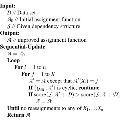
Figure 3: Outline of sequential algorithm for finding the module assignment function

4.2.3 MODULEREASSIGNMENT

In the module reassignment step, the task is more complex. We now have a given structure

S

, and wish to find

A

=argmax_A0scoreM(

S

,

A

0 :

D

). We thus wish to take each variable Xi, and select the

assignment

A

(Xi)that provides the highest score.

At first glance, we might think that we can decompose the score across variables, allowing us to determine independently the optimal assignment

A

(Xi) for each variable Xi. Unfortunately,

this is not the case. Most obviously, the assignments to different variables must be constrained so that the module graph remains acyclic. For example, if X1∈PaMi and X2∈PaMj, we cannot simultaneously assign

A

(X1) = j and

A

(X2) =i. More subtly, the Bayesian score for each module

depends non-additively on the sufficient statistics of all the variables assigned to the module. (The log-likelihood function is additive in the sufficient statistics of the different variables, but the log marginal likelihood is not.) Thus, we can only compute the delta score for moving a variable from one module to another given a fixed assignment of the other variables to these two modules.

We therefore use a sequential update algorithm that reassigns the variables to modules one by one. The idea is simple. We start with an initial assignment function

A

0_{, and in a “round-robin”}

fashion iterate over all of the variables one at a time, and consider changing their module assignment. When considering a reassignment for a variable Xi, we keep the assignments of all other variables

fixed and find the optimal legal (acyclic) assignment for Xi relative to the fixed assignment. We

continue reassigning variables until no single reassignment can improve the score. An outline of this algorithm appears in Figure 3

im-Input:

D // Data set

K // Number of modules Output:

M // A module network Learn-Module-Network

A0= clusterX into K modules S0= empty structure

Loop t=1,2, . . .until convergence

St=Greedy-Structure-Search(At−1,St−1) At=Sequential-Update(At−1,St);

Return M= (At,St)

Figure 4: Outline of the module network learning algorithm. Greedy-Structure-Search successively applies operators that change the structure as long as each such operator results in a legal structure and improves the module network score

prove the score. Hence, it converges to a local maximum, in the sense that no single assignment change can improve the score.

The computation of the score is the most expensive step in the sequential algorithm. Once again, the decomposition of the score plays a key role in reducing the complexity of this computation: When reassigning a variable Xi from one module Mold to another Mnew, only the local scores of

these modules change. The module score of all other modules remains unchanged. The rescoring of these two modules can be accomplished efficiently by subtracting Xi’s statistics from the sufficient

statistics of Mold and adding them to those of Mnew. Thus, assuming that we have precomputed the sufficient statistics associated with every pair of variable Xiand module Mj, the cost of

recom-puting the delta-score for an operator is O(s), where s is the size of the table of sufficient statistics for a module. The only operators whose delta-scores change are those involving reassignment of variables to/from these two modules. Assuming that each module has approximately O(n/K) vari-ables, and we have at most K possible destinations for reassigning each variable, the total number of such operators is generally linear in n. Thus, the cost of each reassignment step is approximately

O(ns). In addition, at the beginning of the module reassignment step, we must initialize all of the sufficient statistics at a cost of O(Mnd), and compute all of the delta-scores at a cost of O(nK).

4.3 Algorithm Summary

To summarize, our algorithm starts with an initial assignment of variables to modules. In general, this initial assignment can come from anywhere, and may even be a random guess. We choose to construct it using the clustering-based idea described in the previous section. The algorithm then iteratively applies the two steps described above: learning the module dependency structures, and re-assigning variables to modules. These two steps are repeated until convergence, where convergence is defined by a score improvement of less than some fixed threshold ∆between two consecutive learned models. An outline of the module network learning algorithm is shown in Figure 4.

1.6 1.3 -1 0.2 1.5 -1.4 -3.5 -2.9 4 -0.2 -3.2 4.1 1.2 1.3 -0.8 0.1 1.1 -1.1 -4 -3.1 3.9 -0.2 -2.9 3.2 1.6 1.3 -1 0.2 1.5 -1.4 -3.5 -2.9 4 -0.2 -3.2 4.1 1.2 1.3 -0.8 0.1 1.1 -1.1 -4 -3.1 3.9 -0.2 -2.9 3.2 x[1] DE LL M SF T A M A T M O T HPQ IN TL x[2] x[3]

x[4] -1.4 1.5 0.2 -1 1.3 1.6 1.2 1.3 -0.8 0.1 1.1 -1.1 -3.5 -2.9 4 -0.2 -3.2 4.1 -4 -3.1 3.9 -0.2 -2.9 3.2 1.6 1.3 -1 0.2 1.5 -1.4 1.2 1.3 -0.8 0.1 1.1 -1.1 -3.5 -2.9 4 -0.2 -3.2 4.1 -4 -3.1 3.9 -0.2 -2.9 3.2 x[1] DE LL M SF T A M A T M O T HPQ IN TL x[3] x[2] x[4] 1

2 0.2 1.5 1.3 1.6 -1.4 -1 4 4.1 -3.5 -2.9 -3.2 -0.2 -0.8 -1.1 1.2 1.3 1.1 0.1 3.9 3.2 -4 -3.1 -2.9 -0.2 -1 -1.4 1.6 1.3 1.5 0.2 4 4.1 -3.5 -2.9 -3.2 -0.2 -0.8 -1.1 1.2 1.3 1.1 0.1 3.9 3.2 -4 -3.1 -2.9 -0.2 x[1] M SF T M O T HPQ DE LL A M A T IN TL x[2] x[3] x[4]

1 2 3

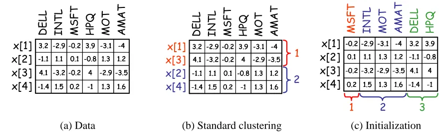
(a) Data (b) Standard clustering (c) Initialization

Figure 5: Relationship between the module network procedure and clustering. Finding an assign-ment function can be viewed as a clustering of the variables whereas clustering typically clusters instances. Shown is sample data for the example domain of Figure 1, where the rows correspond to instances and the columns correspond to variables. (a) Data. (b) Standard clustering of the data in (a). Note that x[2]and x[3]were swapped to form the clusters. (c) Initialization of the assignment function for the module network procedure for the data in (a). Note that variables were swapped in their location to reflect the initial assignment into three modules.

Theorem 4.1: The iterative module network learning algorithm converges to a local maximum of score(

S

,

A

:

D

).

We note that both the structure search step and the module reassignment step are done using simple greedy hill-climbing operations. As in other settings, this approach is liable to get stuck in local maxima. We attempt to somewhat compensate for this limitation by initializing the search at a reasonable starting point, but local maxima are clearly still an issue. An additional strategy that would help circumvent some maxima is the introduction of some randomness into the search (e.g., by random restarts or simulated annealing), as is often done when searching complex spaces with multi-modal target functions.

5. Learning with Regression Trees

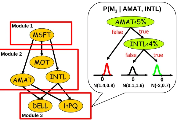
We now briefly review the family of conditional distributions we use in the experiments below. Many of the domains suited for module network models contain continuous valued variables, such as gene expression or price changes in the stock market. For these domains, we often use a condi-tional probability model represented as a regression tree (Breiman et al., 1984). For our purposes, a regression tree T for P(X|U) is defined via a rooted binary tree, where each node in the tree is either a leaf or an interior node. Each interior node is labeled with a test U <u on some variable U∈U and u∈IR. Such an interior node has two outgoing arcs to its children, corresponding to the

outcomes of the test (true or false). The tree structure T captures the local dependency structure of the conditional distribution. The parameters of T are the distributions associated with each leaf. In our implementation, each leaf`is associated with a univariate Gaussian distribution over values of

AMAT<5%

INTL<4%

0 0 0

0 0

false

true false

true

INTL MSFT

MOT

DELL

Module 3 Module 2

Module 1

AMAT

HPQ

P(M₃| AMAT, INTL)

N(1.4,0.8) N(0.1,1.6) N(-2,0.7)

Figure 6: Example of a regression tree with univariate Gaussian distributions at the leaves for rep-resenting the CPD P(M3|AMAT,INTL), associated with M3. The tree has internal nodes

labeled with a test on the variable (e.g. AMAT<5%). Each univariate Gaussian distri-bution at a leaf is parameterized by a mean and a variance. The tree structure captures the local dependency structure of the conditional distributions. In the example shown, when AMAT≥5%, then the distribution over values of variables assigned to M3 will be

Gaussian with mean 1.4 and standard deviation 0.8 regardless of the value of INTL.

Figure 6. We note that, in some domains, Gaussian distributions may not be the appropriate choice of models to assign at the leaves of the regression tree. In such cases, we can apply transforma-tions to the data to make it more appropriate for modeling by Gaussian distributransforma-tions, or use other continuous or discrete distributions at the leaves.

To learn module networks with regression-tree CPDs, we must extend our previous discus-sion by adding another component to

S

that represents the trees T1, . . . ,TK associated with the

dif-ferent modules. Once we specify these components, the above discussion applies with several small differences. These issues are similar to those encountered when introducing decision trees to Bayesian networks (Chickering et al., 1997; Friedman and Goldszmidt, 1998), so we discuss them only briefly.

Given a regression tree Tjfor P(Mj|PaMj), the corresponding sufficient statistics are the statis-tics of the distributions at the leaves of the tree. For each leaf`in the tree, and for each data instance x[m], we let`j[m]denote the leaf reached in the tree given the assignment to PaMjin x[m]. The mod-ule likelihood decomposes as a product of terms, one for each leaf`. Each term is the likelihood for the Gaussian distribution

N

µ`;σ2`

, with the usual sufficient statistics for a Gaussian distribution.

the Gaussian distribution

N

µ`;σ2<sub>`</sub>, with the sufficient statistics for a Gaussian distribution.

ˆ

S0_j,` =

∑

m_Xi

∑

_∈Xj

η{`j[m] =`},

ˆ

S1_j,` =

∑

mXi

∑

∈Xj

η{`j[m] =`}xi, (5)

ˆ

S2_j,` =

∑

mXi

∑

∈Xj

η{`j[m] =`}x2i.

The local module score further decomposes into independent components, one for each leaf

`. Here, we use a Normal-Gamma prior (DeGroot, 1970) for the distribution at each leaf: Letting

τ`=1/σ2` stand for the precision at leaf`, we define: P(µ`,τ`) =P(µ`|τ`)P(τ`), where P(τ`)∼

Γ(α0,β0) and P(µ`|τ`)∼

N

µ0;(λ0τ`)−1, where we assume that all leaves are associated with

the same prior. Letting ˆSi<sub>j,`</sub> be defined as in Equation (5), we have that the component of the log marginal likelihood associated with a leaf`of module j is given by:

−1

2Sˆ

0

j,`log(2π) +

1 2log

λ0

λ0+Sˆ0_j,`

! +log

Γ(α0+

1 2Sˆ

0

j,`)

−log(Γ(α0)) +α0log(β0)−

α0+

1 2Sˆ

0

j,`

log(β),

where

β=β0+

1 2 Sˆ

2

j,`− (Sˆ1<sub>j,`</sub>)2

ˆ

S0_j,`

! +

ˆ

S0_j,`λ0

ˆ

S1

j,`

ˆ

S0j,`

−µ0

2

2(λ0+Sˆ0_j,`)

.

When performing structure search for module networks with regression-tree CPDs, in addition to choosing the parents of each module, we must also choose the associated tree structure. We use the search strategy proposed by Chickering et al. (1997), where the search operators are leaf splits. Such a split operator replaces a leaf in a tree Tj with an internal node with some test on a variable

U . The two branches below the newly created internal node point to two new leaves, each with its

associated Gaussian. This operator must check for acyclicity, as it implicitly adds U as a parent of Mj.

When performing the search, we consider splitting each possible leaf on each possible parent U and each value u. As always in regression-tree learning, we do not have to consider all real values

u as possible split points; it suffices to consider values that arise in the data set. Moreover, under

an appropriate choice of prior (i.e., an independent prior for each leaf), regression-tree learning provides another level of score decomposition: The score of a particular tree is a sum of scores for the leaves in the tree. Thus, a split operation on one leaf in the tree does not affect the score component of another leaf, so that operators applied to other leaves do not need to re-evaluated.

6. Experimental Results

-800 -750 -700 -650 -600 -550 -500 -450

0 20 40 60 80 100 120 140 160 180 200

Number of Modules

T e s t D a ta L o g L ik e li h o o d ( p e r in s ta n c e ) 25 50 100 200 500 -600 -575 -550 -525 -500 -475 -450

0 20 40 60 80 100

Number of modules

T ra in n in g D a ta S c o re ( p e r in s ta n c e ) 25 50 100 200 500 (a) (b)

Figure 7: Performance of learning from synthetic data as a function of the number of modules and training set size. The x-axis corresponds to the number of modules, each curve corre-sponds to a different number of training instances, and each point shows the mean and standard deviations from the 10 sampled data sets. (a) Log-likelihood per instance as-signed to held-out data. (b) Average score per instance on the training data.

to a specification of the total number of modules. We used regression trees as the local probability model for all modules, and uniform priors forρ(

S

)andκ(

A

). For structure search, we used beam search, using a lookahead of three splits to evaluate each operator. When learning Bayesian net-works, as a comparison, we used precisely the same structure learning algorithm, simply treating each variable as its own module.

6.1 Synthetic Data

As a basic test of our procedure in a controlled setting, we used synthetic data generated by a known module network. This gives a known ground truth to which we can compare the learned models. To make the data realistic, we generated synthetic data from a model that was learned from the gene expression data set described below. The generating model had 10 modules and a total of 35 variables that were a parent of some module. From the learned module network, we selected 500 variables, including the 35 parents. We tested our algorithm’s ability to reconstruct the network using different numbers of modules; this procedure was run for training sets of various sizes ranging from 25 instances to 500 instances, each repeated 10 times for different training sets.

10 20 30 40 50 60 70 80 90 100

0 20 40 60 80 100 120 140 160 180 200

Number of Modules

F ra c ti o n o f V a ri a b le s i n 1 0 L a rg e s t M o d u le s 25 50 100 200 500 0 10 20 30 40 50 60 70 80 90

0 20 40 60 80 100 120 140 160 180 200

Number of Modules

R e c o v e re d S tr u c tu re ( % C o rr e c t) 25 50 100 200 500 (a) (b)

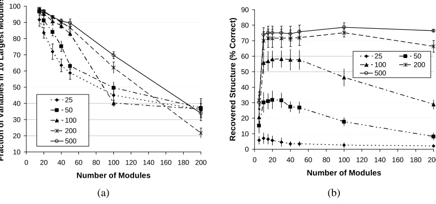
Figure 8: (a) Fraction of variables assigned to the 10 largest modules. (b) Average percentage of correct parent-child relationships recovered (fraction of parent-child relationships in the true model recovered in the learned model) when learning from synthetic data for models with various number of modules and different training set sizes. The x-axis corresponds to the number of modules, each curve corresponds to a different number of training in-stances, and each point shows the mean and standard deviations from the 10 sampled data sets.

To test whether we can use the score of the model to select the number of modules, we also plotted the score of the learned model on the training data (Figure 7(b)). As can be seen, when the number of instances is small (25 or 50), the model with 10 modules achieves the highest score and for a larger number of instances, the score does not improve when increasing the number of modules beyond 10. Thus, these results suggest that we can select the number of modules by choosing the model with the smallest number of modules from among the highest scoring models.

A closer examination of the learned models reveals that, in many cases, they are almost a 10-module network. As shown in Figure 8(a), models learned using 100, 200, or 500 instances and up to 50 modules assigned≥80% of the variables to 10 modules. Indeed, these models achieved high performance in Figure 7(a). However, models learned with a larger number of modules had a wider spread for the assignments of variables to modules and consequently achieved poor performance.

-115.5 -115 -114.5 -114 -113.5 -113

0 5 10 15 20

Algorithm Iterations

S

c

o

re

(

a

v

g

.

p

e

r

g

e

n

e

)

0 10 20 30 40 50

0 5 10 15 20

Algorithm Iterations

G

e

n

e

s

c

h

a

n

g

e

d

(

%

f

ro

m

t

o

ta

l)

Changes from initialization Changes from previous iteration

(a) (b)

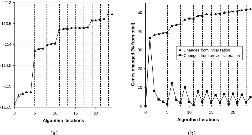
Figure 9: (a) Score of the model (normalized by the number of variables/genes) across the iterations of the algorithm for a module network learned with 50 modules on the gene expression data. Iterations in which the structure was changed are indicated by dashed vertical lines. (b) Changes in the assignment of genes to modules for the module network learned in (a) across the iterations of the algorithm. Shown are both the total changes compared to the initial assignment (triangles) and the changes compared to the previous iteration (squares).

6.2 Gene Expression Data

We next evaluated the performance of our method on a real world data set of gene expression measurements. A microarray measures the activity level (mRNA expression level) of thousands of genes in the cell in a particular condition. We view each experiment as an instance, and the expression level of each measured gene as a variable (Friedman et al., 2000a). In many cases, the coordinated activity of a group of genes is controlled by a small set of regulators, that are themselves encoded by genes. Thus, the activity level of a regulator gene can often predict the activity of the genes in the group. Our goal is to discover these modules of co-regulated genes, and their regulators.

-114.2 -114 -113.8 -113.6 -113.4 -113.2

0 20 40 60 80 100

Runs (initialized from random clusterings)

S

c

o

re

(

a

v

g

.

p

e

r

g

e

n

e

)

Score of model initialization

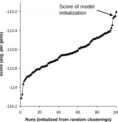
Figure 10: Score of 100 module networks (normalized by the number of variables/genes) each learned with 50 modules from a random clustering initialization, where the runs are sorted according to their score. The score of a module network learned using the de-terministic clustering initialization described in Section 4.2 is indicated by a pointed arrow.

6.2.1 STATISTICALEVALUATION

We first examined the behavior of the learning algorithm on the training data when learning a module network with 50 modules. This network converged after 24 iterations (of which nine were iterations in which the structure of the network changed). To characterize the trajectory of the algorithm, we plot in Figure 9 its improvement across the iterations, measured as the score on the training data, normalized by the number of genes (variables). To obtain a finer-grained picture, we explicitly show structure learning steps, as well as each pass over the variables in the module reassignment step. As can be seen in Figure 9(a), the model score improves nicely across these steps, with the largest gains in score occurring in iterations in which the structure was changed (dotted lines in Figure 9(a)). Figure 9(b) demonstrates how the algorithm changes the assignments of genes to modules, with 1221 of the 2355 (51.8%) genes changing their assignment upon convergence, and the largest assignment changes occurring immediately after structure modification steps.

these sorted scores is shown in Figure 10. Encouragingly, the score for the network initialized using our procedure was better than 97/100 of the runs initialized from random clusters, and the 3/100 runs that did better are only incrementally better.

We evaluated the generalization ability of different models, in terms of log-likelihood of test data, using 10-fold cross validation. In Figure 11(a), we show the difference between module net-works of different size and the baseline Bayesian network, demonstrating that module netnet-works generalize much better to unseen data for almost all choices of number of modules.

6.2.2 BIOLOGICALEVALUATION

As we discussed in the introduction, a common goal in learning a network structure is to reveal structural properties of the underlying distribution. This goal is definitely an important one in the biological domain, where we want to discover both sets of co-regulated genes, and the regulatory mechanism governing their behavior. We therefore evaluated the ability of our module network learning procedure to reveal known biological properties of this domain.

We evaluated a learned module network with 50 modules, where we selected 50 modules due to the biological plausibility of having, on average, 40–50 genes per module. First, we examined whether genes in the same module have shared functional characteristics. To this end, we used annotations of the genes’ biological functions from the Saccharomyces Genome Database (Cherry et

al., 1998). We systematically evaluated each module’s gene set by testing for significantly enriched

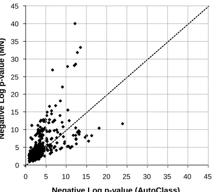
annotations. Suppose we find l genes with a certain annotation in a module of size N. To check for enrichment, we calculate the hypergeometric p-value of these numbers — the probability of finding that many genes of that annotation in a random subset of N genes. For example, the “protein folding” module contains 10 genes, 7 of which are annotated as protein folding genes. In the whole data set, there are only 26 genes with this annotation. The p-value of this annotation, that is, the probability of choosing 7 or more genes in this category by choosing 10 random genes, is less than 10−12. As there are a large number of possible annotations, there is a nontrivial probability that some will be enriched simply by chance. We therefore corrected these p-values using the standard Bonferroni correction for independent multiple hypotheses (Savin, 1980). Our evaluation showed that, of the 50 modules, 42 (resp. 20) modules had at least one significantly enriched annotation with a p-value less than 0.005 (resp. less than 10−6). Furthermore, the enriched annotations reflect the key biological processes expected in our data set. We used these annotations to label the modules with meaningful biological names. A comparison of the overall enrichments of the modules learned by module networks to the enrichments obtained for clusters using AutoClass is shown in Figure 11(b), indicating that there are many annotations that are much more significantly enriched in module networks.

We can use these annotations to reason about the dependencies between different biological processes at the module level. For example, we find that the cell cycle module, regulates the histone module. The cell cycle is the process in which the cell replicates its DNA and divides, and it is indeed known to regulate histones — key proteins in charge of maintaining and controlling the DNA structure. Another module regulated by the cell cycle module is the nitrogen catabolite repression

(NCR) module, a cellular response activated when nitrogen sources are scarce. We find that the NCR

-150 -100 -50 0 50 100 150

0 50 100 150 200 250 300 350 400 450 500

Number of Modules

T e s t D a ta L o g -L ik e li h o o d ( g a in p e r in s ta n c e ) 0 5 10 15 20 25 30 35 40 45

0 5 10 15 20 25 30 35 40 45

Negative Log p-value (AutoClass)

Ne g a ti v e L o g p -v a lu e ( M N )

(a) Test-data generalization (Expression) (b) Annotation enrichment (Expression)

Figure 11: (a) Comparison of generalization ability of module networks learning with different numbers of modules on the gene expression data set. The x-axis denotes the number of modules. The y-axis denotes the difference in log-likelihood on held out data between the learned module network and the learned Bayesian network, averaged over 10 folds; the error bars show the standard deviation. (b) Comparison of the enrichment for anno-tations of functional annoanno-tations between the modules learned using the module network procedure and the clusters learned by the AutoClass clustering algorithm (Cheeseman

et al., 1988) applied to the variables. Each point corresponds to an annotation, and the x

and y axes are the negative log p-values of its enrichment for the two models.

These examples demonstrate the insights that can be gleaned from a higher order model, and which would have been obscured in the unrolled Bayesian network over 2355 genes.

6.3 Stock Market Data

In a very different application, we examined a data set of NASDAQ stock prices. We collected stock prices for 2143 companies, in the period 1/1/2002–2/3/2003, covering 273 trading days (data was obtained fromhttp://finance.yahoo.com). We took each stock to be a variable, and each instance to correspond to a trading day, where the value of the variable is the log of the ratio between that day’s and the previous day’s closing stock price. This choice of data representation focuses on the relative changes to the stock price, and eliminates the magnitude of the price itself (which depends on such irrelevant factors as the number of outstanding shares). As potential controllers, we selected 250 of the 2143 stocks, whose average trading volume was the largest across the data set.

400 450 500 550 600

0 50 100 150 200 250 300

Number of Modules

T e s t D a ta L o g -L ik e li h o o d ( g a in p e r in s ta n c e ) 0 5 10 15 20 25 30 35

0 5 10 15 20 25 30 35

Negative Log p-value (AutoClass)

Ne g a ti v e L o g p -v a lu e ( M N)

(a) Test-data generalization (Stock) (b) Annotation enrichment (Stock)

Figure 12: (a) Comparison of generalization ability of module networks learning with different numbers of modules on the stock data set. The x-axis denotes the number of modules. The y-axis denotes the difference in log-likelihood on held out data between the learned module network and the learned Bayesian network, averaged over 10 folds; the error bars show the standard deviation. (b) Comparison of the enrichment for annotations of sectors between the modules learned using the module network procedure and the clusters learned by the AutoClass clustering algorithm (Cheeseman et al., 1988) applied to the variables. Each point corresponds to an annotation, and the x and y axes are the negative log p-values of its enrichment for the two models.

To test the quality of our modules, we measured the enrichment of the modules in the network with 50 modules for annotations representing various sectors to which each stock belongs (based on sector classifications fromhttp://finance.yahoo.com). We found significant enrichment for 21 such annotations, covering a wide variety of sectors. We also compared these results to the clusters of stocks obtained from applying the popular probabilistic clustering algorithm AutoClass (Cheese-man et al., 1988) to the data. Here, as we described above, each instance corresponds to a stock and is described by 273 random variables, each representing a trading day. In 20 of the 21 cases, the enrichment was far more significant in the modules learned using module networks compared to the one learned by AutoClass, as can be seen in Figure 12(b).