Nonparametric Quantile Estimation

Nonparametric Quantile Estimation

Ichiro Takeuchi [email protected]

Division of Computer Science

Graduate School of Engineering, Mie University 1577, Kurimamachiya-cho, Tsu 514-8507, Japan

Quoc V. Le [email protected]

Timothy D. Sears [email protected]

Alexander J. Smola [email protected]

RSISE, Australian National University and

Statistical Machine Learning Program, National ICT Australia 0200, ACT, Australia

Editor: Chris Williams

Abstract

In regression, the desired estimate of y_|x is not always given by a conditional mean, although

this is most common. Sometimes one wants to obtain a good estimate that satisfies the property that a proportion, τ, of y_|x, will be below the estimate. For τ=0.5 this is an estimate of the

median. What might be called median regression, is subsumed under the term quantile regression.

We present a nonparametric version of a quantile estimator, which can be obtained by solving a simple quadratic programming problem and provide uniform convergence statements and bounds on the quantile property of our estimator. Experimental results show the feasibility of the approach and competitiveness of our method with existing ones. We discuss several types of extensions including an approach to solve the quantile crossing problems, as well as a method to incorporate prior qualitative knowledge such as monotonicity constraints.

Keywords: support vector machines, kernel methods, quantile estimation, nonparametric tech-niques, estimation with constraints

1. Introduction

Regression estimation is typically concerned with finding a real-valued function f such that its values f(x) correspond to the conditional mean of y, or closely related quantities. Many methods have been developed for this purpose, e.g. least mean square (LMS) regression, robust regression (Huber, 1981), orε-insensitive regression (Vapnik, 1995; Vapnik et al., 1997). Regularized variants include Wahba (1990), penalized by a Reproducing Kernel Hilbert Space (RKHS) norm, and Hoerl and Kennard (1970), regularized via ridge regression.

1.1 Motivation

• A device manufacturer may wish to know what are the 10% and 90% quantiles for some feature of the production process, so as to tailor the process to cover 80% of the devices produced.

• For risk management and regulatory reporting purposes, a bank may need to estimate a lower bound on the changes in the value of its portfolio which will hold with high probability.

• A pediatrician requires a growth chart for children given their age and perhaps even med-ical background, to help determine whether medmed-ical interventions are required, e.g. while monitoring the progress of a premature infant.

These problems are addressed by a technique called Quantile Regression (QR) or Quantile Estima-tion championed by Koenker (see Koenker, 2005, for a descripEstima-tion, practical guide, and extensive list of references). These methods have been deployed in econometrics, social sciences, ecology, etc. The purpose of our paper is:

• To bring the technique of quantile regression to the attention of the machine learning commu-nity and show its relation toν-Support Vector Regression (Sch¨olkopf et al., 2000).

• To demonstrate a nonparametric version of QR which outperforms the currently available nonlinear QR regression formations (Koenker, 2005). See Section 5 for details.

• To derive small sample size results for the algorithms. Most statements in the statistical literature for QR methods are of asymptotic nature (Koenker, 2005). Empirical process results permit us to define two quality criteria and show tail bounds for both of them in the finite-sample-size case.

• To extend the technique to permit commonly desired constraints to be incorporated. As exam-ples we show how to enforce non-crossing constraints and a monotonicity constraint. These constraints allow us to incorporate prior knowlege on the data.

1.2 Notation and Basic Definitions

In the following we denote by

X

Y

training set with corresponding targets Y =_{y1, . . . ,ym}, both drawn independently and identically

distributed (iid) from some distribution p(x,y). With some abuse of notation y also denotes the vector of all yiin matrix and vector expressions, whenever the distinction is obvious.

Unless specified otherwise

H

X

denotes a vector in feature space andφ(x)is the corresponding feature map of x. That is, k(x,x′) = hφ(x),φ(x′)_i. Finally,α_∈Rmis the vector of Lagrange multipliers.

Definition 1 (Quantile) Denote by y_∈Ra random variable and letτ_∈(0,1). Then theτ-quantile

of y, denoted by µ_τis given by the infimum over µ for which Pr_{y_≤µ_}=τ. Likewise, the conditional

quantile µτ(x)for a pair of random variables(x,y)_∈

X

X

1.3 Examples

To illustrate regression analyses with conditional quantile functions, we provide two simple exam-ples here.

1.3.1 ARTIFICIALDATA

The above definition of conditional quantiles may be best illustrated by a simple example. Consider a situation where the relationship between x and y is represented as

y(x) = f(x) +ξ, whereξ_∼

N

. (1)

Here, note that, the amount of noiseξis a function of x. Sinceξis symmetric with mean and median 0 we have µ0.5(x) = f(x). Moreover, we can compute theτ-th quantiles by solving Pr{y≤µ|x}=

τ explicitly. Since ξ is normally distributed, we know that the τ-th quantile of ξ is given by σ(x)Φ−1₍τ_{), where} Φ_{is the cumulative distribution function of the normal distribution with unit} variance. This means that

µτ(x) = f(x) +σ(x)Φ−1(τ).

Figure 1 shows the case where x is uniformly drawn from [₋1,1]and y is obtained based on (1) with f(x) =sinc(x)andσ(x) =0.1 exp(1₋x). The black circles are 500 data examples and the five curves areτ=0.10,0.25,0.50,0.75 and 0.90 conditional quantile functions. The probability densities p(y_|x=₋0.5)and p(y_|x= +0.5)are superimposed. Theτ-th conditional quantile function is obtained by connecting theτ-th quantile of the conditional distribution p(y_|x)for all x_∈

X

1.3.2 REALDATA

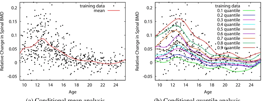
The next example is based on actual measurements of bone density (BMD) in adolescents. The data was originally reported in Bachrach et al. (1999) and is also analyzed in Hastie et al. (2001).1 Figure 2 (a) shows a regression analysis with conditional mean and figure 2 (b) shows that with a set of conditional quantiles for the variable BMD. The response in the vertical axis is relative change in spinal BMD and the covariate in the horizontal axis is the age of the adolescents. The conditional mean analysis (a) provides only the central tendency of the conditional distribution, while apparently the entire distribution of BMD changes according to age. The conditional quantile analysis (b) gives us more detailed description of these changes. For example, we can see that the variance of the BMD changes with the age (heteroscedastic) and that the conditional distribution is slightly positively skewed.

2. Quantile Estimation

Given the definition of µτ(x)and knowledge of support vector machines we might be tempted to use version of theε-insensitive tube regression to estimate µ_τ(x). More specifically one might try to

-2 -1.5 -1 -0.5 0 0.5 1 1.5 2

-1 -0.5 0 0.5 1

data sample 0.10 quantile 0.25 quantile 0.50 quantile 0.75 quantile 0.90 quantile data sample 0.10 quantil 0.25 quantil 0.50 quantil 0.75 quantil 0.90 quantil

py^x

py^x

input x

output

y

Figure 1: Illustration of conditional quantile functions of a simple artificial system in (1) with

f(x) =sinc(x)andσ(x) =0.1 exp(1₋x). The black circles are 500 data examples and the five curves areτ=0.10,0.25,0.50,0.75 and 0.90 conditional quantile functions. The probability densities p(y_|x=₋0.5)and p(y_|x= +0.5)are superimposed. In this paper, we are concerned with the problem of estimating these conditional quantile functions from training data.

estimate quantiles nonparametrically using an extension of theν-trick, as outlined in Sch¨olkopf et al. (2000). However this approach carries the disadvantage of requiring us to estimate both an upper and lower quantile simultaneously.2_{While this can be achieved by quadratic programming, in doing} so we estimate “too many” parameters simultaneously. More to the point, if we are interested in finding an upper bound on y which holds with 0.95 probability we may not want to use information about the 0.05 probability bound in the estimation. Following Vapnik’s paradigm of estimating only the relevant parameters directly (Vapnik, 1982) we attack the problem by estimating each quantile separately. For completeness and comparison, we provide a detailed description of a symmetric quantile regression in Appendix A.

2.1 Loss Function

The basic strategy behind quantile estimation arises from the observation that minimizing theℓ1-loss function for a location estimator yields the median. Observe that to minimize∑m_i=1|yi−µ|by choice

of µ, an equal number of terms yi−µ have to lie on either side of zero in order for the derivative wrt.

µ to vanish. Koenker and Bassett (1978) generalizes this idea to obtain a regression estimate for any

quantile by tilting the loss function in a suitable fashion. More specifically one may show that the following “pinball” loss leads to estimates of theτ-quantile:

Lemma 2 (Quantile Estimator) Let Y =_{y1, . . . ,ym} ⊂Rand letτ∈(0,1)then the minimizer µτ

of∑m_i=1lτ(yi−µ)with respect to µ satisfies:

-0.05 0 0.05 0.1 0.15 0.2

10 12 14 16 18 20 22 24

Relative

Cha

nge in S

pinal B

MD

Age

training data mean

-0.05 0 0.05 0.1 0.15 0.2

10 12 14 16 18 20 22 24

Relative

Cha

nge in S

pinal B

MD

Age

training data 0.1 quantile 0.2 quantile 0.3 quantile 0.4 quantile 0.5 quantile 0.6 quantile 0.7 quantile 0.8 quantile 0.9 quantile

(a) Conditional mean analysis (b) Conditional quantile analysis

Figure 2: An illustration of (a) conditional mean analysis and (b) conditional quantile analysis for a data set on bone mineral density (BMD) in adolescents. In (a) the conditional mean curve is estimated by regression spline with least square criterion. In (b) the nine curves are the estimated conditional quantile curves at orders 0.1,0.2, . . . ,0.9. The set of conditional quantile curves provides more informative description of the relationship among variables such as non-constant variance or non-normality of the noise (error) distribution. In this paper, we are concerned with the problem of estimating these conditional quantiles.

lτ(ξ) =

(

τξ ifξ_≥0

(τ₋1)ξ ifξ<0 (2)

0

0

ξ

l

τ(ξ)

τ

τ − 1

Figure 3: Pinball loss function for quantile estimation.

1. The number of terms, m₋, with yi<µτis bounded from above byτm.

2. The number of terms, m+, with yi>µτis bounded from above by(1−τ)m.

3. For m_→∞, the fraction m−

m, converges toτif Pr(y)does not contain discrete components.

Proof Assume that we are at an optimal solution. Then, increasing the minimizer µ byδµ changes

opti-mality in conjunction with the fact that m₋+m+≤m proves the first two claims. To see the last claim, simply note that the event yi=yjfor i6=j has probability measure zero for distributions not

containing discrete components. Taking the limit m_→∞shows the claim.

The idea is to use the same loss function for functions, f(x), rather than just constants in order to obtain quantile estimates conditional on x. Koenker (2005) uses this approach to obtain linear estimates and certain nonlinear spline models. In the following we will use kernels for the same purpose.

2.2 Optimization Problem

Based on l_τ(ξ)we define the expected quantile risk as

R[f]:=Ep(x,y)[lτ(y−f(x))]. (3)

By the same reasoning as in Lemma 2 it follows that for f :

X

minimizing the empirical risk plus a regularizer:

Rreg[f]:=

1

m

m

∑

i=1

l_τ(yi−f(xi)) +

λ 2kgk

2

H where f =g+b and b∈R. (4)

Here_k·kH is RKHS norm and we require g∈

H

offset, b, in the optimization problem. This ensures that the minimizer of (4) will satisfy the quantile property:

Lemma 3 (Empirical Conditional Quantile Estimator) Assuming that f contains a scalar

un-regularized term, the minimizer of (4) satisfies:

1. The number of terms m₋with yi< f(xi)is bounded from above byτm.

2. The number of terms m+with yi> f(xi)is bounded from above by(1−τ)m.

3. If (x,y) is drawn iid from a distribution Pr(x,y), with Pr(y_|x) continuous and the

expecta-tion of the modulus of absolute continuity of its density satisfying lim_δ→0E[ε(δ)] =0. With

probability 1, asymptotically, m−

m equalsτ.

Proof For the two claims, denote by f∗the minimum of Rreg[f]with f∗=g∗+b∗. Then Rreg[g∗+b] has to be minimal for b=b∗. With respect to b, however, minimizing Rregamounts to finding theτ quantile in terms of yi−g(xi). Application of Lemma 2 proves the first two parts of the claim.

For the second part, an analogous reasoning to Sch¨olkopf et al. (2000, Proposition 1) applies. In a nutshell, one uses the fact that the measure of theδ-neighborhood of f(x)converges to 0 for δ→0. Moreover, for kernel functions the entropy numbers are well behaved (Williamson et al., 2001). The application of the union bound over a cover of such function classes completes the proof. Details are omitted, as the proof is identical to that of Sch¨olkopf et al. (2000).

Later, in Section 4 we discuss finite sample size results regarding the convergence of m−

m →τand

2.3 Dual Optimization Problem

Here we compute the dual optimization problem to (4) for efficient numerical implementation. Us-ing the connection between RKHS and feature spaces we write f(x) =_hφ(x),w_i+b and we obtain

the following equivalent to minimizing Rreg[f]. minimize

w,b,ξ(∗)i

C

m

∑

i=1

τξi+ (1−τ)ξ∗i +

1 2kwk

2 _(5a)

subject to yi− hφ(xi),wi −b≤ξiandhφ(xi),wi+b−yi≤ξi∗whereξi,ξ∗i ≥0 (5b)

Here we used C :=1/(λm). The dual of this problem can be computed straightforwardly using Lagrange multipliers. The dual constraints for ξandξ∗ can be combined into one variable. This yields the following dual optimization problem

minimize

α

1 2α

⊤_Kα−α⊤_{~y subject to C(τ−1)≤α}

i≤Cτfor all 1≤i≤m and~1⊤α=0. (6)

We recover f via the familiar kernel expansion

w=

∑

i

αiφ(xi)or equivalently f(x) =

∑

αik(xi,x) +b. (7)

Note that the constant b is the dual variable to the constraint 1⊤α=0. Alternatively, b can be obtained by using the fact that f(xi) =yiforαi6∈ {C(τ−1),Cτ}. The latter holds as a consequence

of the KKT-conditions on the primal optimization problem of minimizing Rreg[f].

Note that the optimization problem is very similar to that of anε-SV regression estimator (Vap-nik et al., 1997). The key difference between the two estimation problems is that inε-SVR we have an additionalε_kα_k1penalty in the objective function. This ensures that observations with deviations from the estimate, i.e. with_|yi−f(xi)|<εdo not appear in the support vector expansion. Moreover

the upper and lower constraints on the Lagrange multipliersαi are matched. This means that we

balance excess in both directions. The latter is useful for a regression estimator. In our case, how-ever, we obtain an estimate which penalizes loss unevenly, depending on whether f(x)exceeds y or vice versa. This is exactly what we want from a quantile estimator: by this procedure errors in one direction have a larger influence than those in the converse direction, which leads to the shifted esti-mate we expect from QR. A practical advantage of (6) is that it can be solved directly with standard quadratic programming code rather than using pivoting, as is needed in SVM regression (Vapnik et al., 1997).

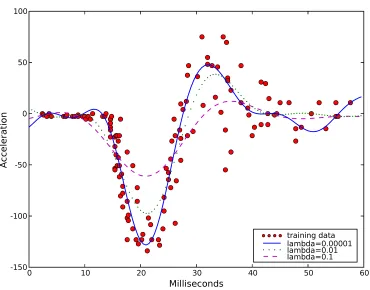
A practical estimate does require a procedure for setting the regularization parameter. Figure 4 shows how QR responds to changing the regularization parameter. All three estimates in Figure 4 attempt to compute the median, subject to different smoothness constraints. While they all satisfy the quantile property having half the points on either side of the regression, some estimates appear track the observations better. This issue is addressed in Section 5 where we compute quantile regression estimates on a range of data sets.

3. Extensions and Modifications

0 1 0 2 0 3 0 4 0 5 0 6 0

M illis e c o n d s

1 5 0

1 0 0

5 0

0

5 0 1 0 0

Ac

c

e

l

e

r

a

t

io

n

tra in in g d a ta

l

a m b d a =

0 .0 0 0 0 1

l

a m b d a =

0 .0 1

l

a m b d a =

0 .1

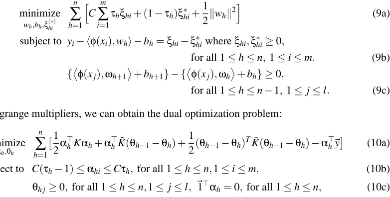
3.1 Non-Crossing Constraints

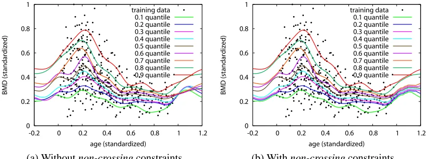
When we want to estimate several conditional quantiles (e.g. τ=0.1,0.2, . . . ,0.9), two or more estimated conditional quantile functions can cross or overlap. This embarrassing phenomenon called quantile crossings occurs because each conditional quantile function is independently es-timated (Koenker, 2005; He, 1997). Figure 5(a) shows BMD data presented in 1.3.2 and τ= 0.1,0,2, . . . ,0.9 conditional quantile functions estimated by the kernel-based estimator described in the previous section. Both of the input and the output variables are standardized in [0,1]. We note quantile crossings at several places, especially at the outside of the training data range (x<0 and 1<x). In this subsection, we address this problem by introducing non-crossing constraints.3

Figure 5(b) shows a family of conditional quantile functions estimated with the non-crossing con-straints.

Suppose that we want to estimate n conditional quantiles at 0<τ1 <τ2< . . . <τn<1. We

enforce non-crossing constraints at l points_{xj}lj=1in the input domain

X

H

non-crossing constraints are represented as linear constraints

φ

(xj),ωh

+bh≤

φ

(xj),ωh+1

+bh+1, for all 1≤h≤n−1,1≤ j≤l. (8) Solving (5) or (6) for 1_≤h_≤n with non-crossing constraints (8) allows us to estimate n conditional

quantile functions not crossing at l points x1, . . . ,xl ∈

X

by

minimize

wh,bh,ξ(∗)hi

n

∑

h=1

h

C

m

∑

i=1

τhξhi+ (1−τh)ξ∗hi+

1 2kwhk

2i _(9a)

subject to yi− hφ(xi),whi −bh=ξhi−ξ∗hiwhereξhi,ξ∗hi≥0,

for all 1_≤h_≤n,1_≤i_≤m. (9b) {φ

(xj),ωh+1

+bh+1} − {

φ

(xj),ωh

+bh} ≥0,

for all 1≤h≤n−1,1≤ j≤l. (9c)

Using Lagrange multipliers, we can obtain the dual optimization problem:

minimize

αh,θh

n

∑

h=1

1

2α

⊤

hKαh+α⊤hK˜(θh−1−θh) +

1

2(θh−1−θh)

T_K¯(θ

h−1−θh)−α⊤h~y

(10a)

subject to C(τh−1)≤αhi≤Cτh, for all 1≤h≤n,1≤i≤m, (10b)

θh j≥0,for all 1≤h≤n,1≤j≤l, ~1⊤αh=0,for all 1≤h≤n, (10c)

whereθh jis the Lagrange multiplier of (9c) for all 1≤h≤n, 1≤ j≤l, ˜K is m×l matrix with its

(i,j)-th entry k(xi,xj), ¯K is l×l matrix with its(j1,j2)-th entry k(xj1,xj2)andθhis l-vector with its

j-th entryθh jfor all 1≤h≤n. For notational convenience we defineθ0 j=θn j=0 for all 1≤j≤l.

The model for conditional quantileτh-th quantile function is now represented as

fh(x) =

m

∑

i=1

αhik(x,xi) + l

∑

j=1

(θh−1i−θhi)k(x,xj) +bh. (11)

In section 5.2.1 we empirically investigate the effect of non-crossing constraints on the generaliza-tion performances.

It is worth noting that, after enforcing the non-crossing constraints, the quantile property as in Lemma 3 may not be guaranteed. This is because the method both tries to optimize for the quantile property and the non-crossing property (in relation to other quantiles). Hence, the final outcome may not empirically satisfy the quantile property. Yet, the non-crossing constraints are very nice because they ensure the semantics of the quantile definition: lower quantile level should not cross the higher quantile level.

0 0.2 0.4 0.6 0.8 1

-0.2 0 0.2 0.4 0.6 0.8 1 1.2

BMD (standardized

)

age (standardized) training data

0.1 quantile 0.2 quantile 0.3 quantile 0.4 quantile 0.5 quantile 0.6 quantile 0.7 quantile 0.8 quantile 0.9 quantile

0 0.2 0.4 0.6 0.8 1

-0.2 0 0.2 0.4 0.6 0.8 1 1.2

BMD (standardized

)

age (standardized) training data

0.1 quantile 0.2 quantile 0.3 quantile 0.4 quantile 0.5 quantile 0.6 quantile 0.7 quantile 0.8 quantile 0.9 quantile

(a) Without non-crossing constraints (b) With non-crossing constraints

Figure 5: An example of quantile crossing problem in BMD data set presented in Section 1. Both of the input and the output variable are standardized in[0,1]. In (a) the set of conditional quantiles at 0.1,0.2, . . . ,0.9 are estimated by the kernel-based estimator presented in the previous section. Quantile crossings are found at several points, especially at the outside of the training data range (x<0 and 1<x). The plotted curves in (b) are the conditional

quantile functions obtained with non-crossing constraints explained in Section 3.1. There are no quantile crossing even at the outside of the training data range.

3.2 Monotonicity and Growth Curves

Consider the situation of a health statistics office which wants to produce growth curves. That is, it wants to generate estimates of y being the height of a child given parameters x such as age, ethnic background, gender, parent’s height, etc. Such curves can be used to assess whether a child’s growth is abnormal.

A naive approach is to apply QR directly to the problem of estimating y_|x. Note, however, that

50 100 150 200

5

10 15 20 25 30 35 40 45 50

Figure 6: Example plots from quantile regression with and without monotonicity constraints. The thin line represents the nonparametric quantile regression without monotonicity con-straints whereas the thick line represents the nonparamtric quantile regression with mono-tonicity constraints.

To address this problem we adopt an approach similar to (Vapnik et al., 1997; Smola and Sch¨olkopf, 1998) and impose constraints on the derivatives of f directly. While this only ensures that f is monotonic on the observed data X , we could always add more locations x′_ifor the express purpose of enforcing monotonicity.

Formally, we require that for a differential operator D, such as D=∂xage the estimate D f(x)≥0

for all x_∈X . Using the linearity of inner products we have

D f(x) =D(hφ(x),wi+b) =hDφ(x),wi=hψ(x),wi whereψ(x):=Dφ(x). (12)

constraints and we need to solve

minimize

w,b,ξi

C

m

∑

i=1

τξi+ (1−τ)ξ∗i +

1 2kwk

2

subject to yi− hφ(xi),wi −b≤ξi, hφ(xi),wi+b−yi≤ξ∗i,

hψ(xi),wi ≥0, ξi,ξ∗i ≥0.

Since the additional constraint does not depend on b it is easy to see that the quantile property still holds. The dual optimization problem yields

minimize

α,β

1 2

α

β

⊤

K D1K

D2K D1D2K

α β

−α⊤~y (13a)

subject to C(τ₋1)_≤αi≤Cτand 0≤βifor all 1≤i≤m and~1⊤α=0. (13b)

Here D1K is a shorthand for the matrix of entries D1k(xi,xj)and D2K,D1D2K are defined analo-gously. Here w=∑_iαiφ(xi) +βiψ(xi)or equivalently f(x) =∑iαik(xi,x) +βiD1k(xi,x) +b.

Example Assume that x_∈Rn and that x1 is the coordinate with respect to which we wish to enforce monotonicity. Moreover, assume that we use a Gaussian RBF kernel, that is

k(x,x′) =exp

− 1 2σ2

x−x′

2

. (14)

In this case D1=∂1with respect to x and D2=∂1with respect to x′. Consequently we have

D1k(x,x′) =

x′₁₋x1

σ2 k(x,x

′_{); D}

2k(x,x′) =

x1−x′₁

σ2 k(x,x

′_{) (15a)}

D1D2k(x,x′) =

"

σ−2

−(x1−x′1) 2 σ4

#

k(x,x′). (15b)

Plugging the values of (15) into (13) yields the quadratic program. Note also that both k(x,x′)and

D1k(x,x′)in (15a), are used in the function expansion.

If x1 were drawn from a discrete (yet ordered) domain we could replace D1,D2 with a finite difference operator. This is still a linear operation on k and consequently the optimization problem remains unchanged besides a different functional form for D1k.

An alternative to the above approach is not to modify the optimization problem but to ensure the constraints by modifying the function in the hypothesis space which is much simpler to implement as in Le et al. (2006).

3.3 Other Function Classes

Semiparametric Estimates RKHS expansions may not be the only function classes desired for quantile regression. For instance, in the social sciences a semiparametric model may be more de-sirable, as it allows for interpretation of the linear coefficients (Gu and Wahba, 1993; Smola et al., 1999; Bickel et al., 1994). In this case we add a set of parametric functions fiand solve

minimize 1

m

m

∑

i=1

lτ(yi−f(xi)) +

λ 2kgk

2

H where f(x) =g(x) + n

∑

i=1

For instance, the function class fi could be linear coordinate functions, that is, fi(x) =xi. The

main difference to (6) is that the resulting optimization problem exhibits a larger number of equality constraint. We obtain (6) with the additional constraints

m

∑

j=1

αjfi(xj) =0 for all i. (17)

Linear Programming Regularization Convex function classes withℓ1penalties can be obtained by imposing an_kα_k1penalty instead of the_kg_k2_H penalty in the optimization problem. The advan-tage of this setting is that minimizing

minimize 1

m

m

∑

i=1

l_τ(yi−f(xi)) +λ

n

∑

j=1

|αi|where f(x) = n

∑

i=1

αifi(x) +b. (18)

is a linear program which can be solved efficiently by existing codes for large scale problems. In the context of (18) the functions ficonstitute the generators of the convex function class. This approach

is similar to Koenker et al. (1994) and Bosch et al. (1995). The former discussℓ1regularization of expansion coefficients whereas the latter discuss an explicit second order smoothing spline method for the purpose of quantile regression. Most of the discussion in the present paper can be adapted to this case without much modification. For details on how to achieve this see Sch¨olkopf and Smola (2002). Note that smoothing splines are a special instance of kernel expansions where one assumes explicit knowledge of the basis functions.

Relevance Vector Regularization and Sparse Coding Finally, for sparse expansions one can use more aggressive penalties on linear function expansions than those given in (18). For instance, we could use a staged regularization as in the RVM (Tipping, 2001), where a quadratic penalty on each coefficient is exerted with a secondary regularization on the penalty itself. This corresponds to a Student-t penalty onα.

Likewise we could use a mix between an ℓ1 andℓ0 regularizer as used in Fung et al. (2002) and apply successive linear approximation. In short, there exists a large number of regularizers, and (non)parametric families which can be used. In this sense the RKHS parameterization is but one possible choice. Even so, we show in Section 5 that QR using the RKHS penalty yields excellent performance in experiments.

Neural Networks, Generalized Models Our method does not depend on the how the function class is represented (not only the Kernelized version), in fact, one can use Neural Networks or Generalized Models for estimation as long as the loss function is kept the same. This is the main reason why this paper is called Non-parametric quantile estimation.

4. Theoretical Analysis

In this section we state some performance bounds for our estimator.

4.1 Performance Indicators

• fτneeds to satisfy the quantile property as well as possible. That is, we want that Pr

X,Y{|Pr{y<fτ(x)} −τ| ≥ε} ≤δ. (19)

In other words, we want that the probability that y< f_τ(x)does not deviate fromτby more thanεwith high probability, when viewed over all draws(X,Y)of training data. Note how-ever, that (19) does not imply having a conditional quantile estimator at all. For instance, the constant function based on the unconditional quantile estimator with respect to Y performs extremely well under this criterion. Hence we need a second quantity to assess how closely

fτ(x)tracks µτ(x).

• Since µ_τ itself is not available, we take recourse to (3) and the fact that µ_τ is the minimizer of the expected risk R[f]. While this will not allow us to compare µτand fτdirectly, we can at least compare it by assessing how close to the minimum R[f_τ∗]the estimate R[f_τ]is. Here

f_τ∗is the minimizer of R[f]with respect to the chosen function class. Hence we will strive to bound

Pr

X,Y{R[fτ]−R[f ∗

τ]>ε} ≤δ. (20)

These statements will be given in terms of the Rademacher complexity of the function class of the estimator as well as some properties of the loss function used in select it. The technique itself is standard and we believe that the bounds can be tightened considerably by the use of localized Rademacher averages (Mendelson, 2003), or similar tools for empirical processes. However, for the sake of simplicity, we use the tools from Bartlett and Mendelson (2002), as the key point of the derivation is to describe a new setting rather than a new technique.

4.2 Bounding R[f_τ∗]

Definition 4 (Rademacher Complexity) Let X :=_{x1, . . . ,xm}be drawn iid from p(x)and let

F

be a class of functions mapping from(X)toR. Letσibe independent uniform{±1}-valued random

variables. Then the Rademacher complexity

R

R

ˆ

R

F

sup

f∈F 2 m n

∑

σif(xi) X i

and

R

F

h

ˆ

R

F

. (21)

Conveniently, if Φ is a Lipschitz continuous function with Lipschitz constant L, one can show (Bartlett and Mendelson, 2002) that

R

F

R

F

F

F

An analogous result exists for empirical quantities bounding ˆ

R

F

R

F

Theorem 5 (Concentration for Lipschitz Continuous Functions) For any Lipschitz continuous

function Φ with Lipschitz constant L and a function class

F

X

probability measure on

X

X

sup

f_∈F

Ex[Φ(f(x))]−

1

m

m

∑

i=1

Φ(f(xi))

≤2L

R

F

r

8 log 2/δ

We can immediately specialize the theorem to the following statement about the loss for QR:

Theorem 6 Denote by f_τ∗ the minimizer of the R[f]with respect to f _∈

F

all f _∈

F

sample size m and 0<δ<1, every quantile regression estimate f_τsatisfies with probability at least

(1₋δ)

R[fτ]−R[f_τ∗]_≤2 max L

R

F

r

log 2/δ

2m where L={τ,1−τ}. (24)

Proof We use the standard bounding trick that

R[f_τ]₋R[f_τ∗]_≤

R[fτ]−R_emp[fτ]

+R_emp[fτ∗]−R[fτ∗] (25)

≤sup

f∈F

R[f]−R_emp[f]

+R_emp[fτ∗]−R[fτ∗] (26)

where (25) follows from Remp[fτ]≤Remp[f_τ∗]. The first term can be bounded directly by The-orem 5. For the second part we use Hoeffding’s bound (Hoeffding, 1963) which states that the

deviation between a bounded random variable and its expectation is bounded by B

q

log 1/δ 2m with probabilityδ. Applying a union bound argument for the two terms with probabilities 2δ/3 andδ/3 yields the confidence-dependent term. Finally, using the fact that lτ is Lipschitz continuous with

L=max(τ,1₋τ)completes the proof.

Example Assume that

H

F

Mendel-son (2003) that

R

F

convergence of

R[f_τ]₋R[f_τ∗] =O(m−12). (27)

This is as good as it gets for nonlocalized estimates. Since we do not expect R[f]to vanish except for pathological applications where quantile regression is inappropriate (that is, cases where we have a deterministic dependency between y and x), the use of localized estimates (Bartlett et al., 2002) provides only limited returns. We believe, however, that the constants in the bounds could benefit from considerable improvement.

4.3 Bounds on the Quantile Property

The theorem of the previous section gave us some idea about how far the sample average quantile loss is from its true value under p. We now proceed to stating bounds to which degree f_τ satisfies the quantile property, i.e. (19).

In this view (19) is concerned with the deviation Eχ(−∞,0](y−fτ(x))

r+_ε (ξ):=min{1,max{0,1−ξ/ε_}} (28a)

r−_ε (ξ):=min_{1,max_{0,₋ξ/ε_}} (28b)

0 1

0 lower

bound

upper bound

ε

−ε ξ

rε- (ξ) rε+ (ξ)

Figure 7: Ramp functions bracketing the characteristic function via r+_{ε ≥}χ_{(−∞,0]≥}r_ε−.

Theorem 7 Under the assumptions of Theorem 6 the expected quantile is bounded with probability

1₋δeach from above and below by

1

m

m

∑

i=1

r_ε−(yi−f(xi))−∆≤E

χ

(−∞,0](y−fτ(x))

≤ 1

m

m

∑

i=1

r+_ε(yi−f(xi)) +∆, (29)

where the statistical confidence term is given by∆=2

ε

R

F

q −8 logδ

m .

Proof The claim follows directly from Theorem 5 and the Lipschitz continuity of r+_ε and r−_ε. Note that r+_ε and r−_ε minorize and majorize ξ_(−∞,0], which bounds the expectations. Next use a Rademacher bound on the class of loss functions induced by r_ε+◦

F

F

Note that Theorem 7 allows for some flexibility: we can decide to use a very conservative bound in terms ofε, i.e. a large value of ε to reap the benefits of having a ramp function with small L. This leads to a lower bound on the Rademacher average of the induced function class. Likewise, a smallεamounts to a potentially tight approximation of the empirical quantile, while risking loose statistical confidence terms.

5. Experiments

The present section mirrors the theoretical analysis of the previous section.

5.1 Experiments with Standard Nonparametric Quantile Regression

We check the performance of various quntile estimators with respect to two criteria:

• Simultaneously we need to ensure that the estimate satisfies the quantile property, that is, we want to ensure that the estimator we obtained does indeed produce numbers fτ(x)which exceed y with probability close toτ. The quantile property was measured by ramp loss.4 5.1.1 MODELS

We compare the following four models:

• An unconditional quantile estimator. Given the simplicity of the function class (constants!) this model should tend to underperform all other estimates in terms of minimizing the em-pirical risk. By the same token, it should perform best in terms of preserving the quantile property. This appears asuncond.

• Linear QR as described in Koenker and Bassett (1978). This uses a linear unregularized model to minimize l_τ. In experiments, we used the rqroutine available in the R package5 calledquantreg. This appears aslinear.

• Nonparametric QR as described by Koenker et al. (1994). This uses a spline model for each coordinate individually, with linear effect. The fitting routine used wasrqss, also available

in quantreg.6 The regularization parameter in this model was chosen by 10-fold

cross-validation within the training sample. This appears asrqss.

• Nonparametric quantile regression as described in Section 2. We used Gaussian RBF ker-nels with automatic kernel width (ω2) and regularization (C) adjustment by 10-fold cross-validation within training sample.7 This appears asnpqr.

As we increase the complexity of the function class (from constant to linear to nonparametric) we expect that (subject to good capacity control) the expected risk will decrease. Simultaneously we expect that the quantile property becomes less and less maintained, as the function class grows. This is exactly what one would expect from Theorems 6 and 7. As the experiments show, performance of thenpqrmethod is comparable or significantly better than other models. In particular it preserves the quantile property well.

Notes on Gaussian RBF kernel parameter selection trick The parameter σ in the Gaussian kernel could be chosen by the following trick. We fist subsample the training data (if the training data set is not large, use the whole training data), then compute the distance between the points and find the distances at 0.9 and 0.1 quantile of all the distances, the average distance of these two distances is set to be the initialσ0. This is to guarantee that the kernel parameter is neither too big or too small. Other values ofσto be selected in the experiments (via cross-validation) are [10−4_σ

0, . . . ,σ0, . . . ,103σ0,104σ0]. In general, depending on the problems, one may set the search space to be finer (the distance between two consecutive items in the list is smaller) or coarser (the distance between two consecutive items in the list is larger), or even a higher value for maximum item in the list, and a smaller value for minimum item in the list, etc.

4. In the experiments we setε=0 in (28) for simplicity. Thus, it might be appropriate to call it as step loss rather than ramp loss. However, we keep to use the term “ramp loss” throughout this paper.

5. See http://cran.r-project.org/.

6. Additional code containing bugfixes and other operations necessary to carry out our experiments is available at http://users.rsise.anu.edu.au/∼timsears.

5.1.2 DATASETS

We chose 20 regression data sets from the following R packages:mlbench, quantreg, alr3and

MASS. The first library contains data sets from the UCI repository. The last two were made available as illustrations for regression textbooks. The data sets are all documented and available in R. Data sets were chosen not to have any missing variables, to have suitable datatypes, and to be of a size where all models would run on them.8In most cases either there was an obvious variable of interest, which was selected as the y-variable, or else we chose a continuous variable arbitrarily. The sample sizes vary from m=38 (CobarOre) to m=1375 (heights), and the number of regressors vary from

d=1 (5 sets) and d =12 (BostonHousing). Some of the data sets contain categorical variables. We omitted variables which were effectively record identifiers, or obviously produced very small groupings of records. Finally, we standardized all data sets coordinatwise to have zero mean and unit variance before running the algorithms. This had a side benefit of putting the pinball loss on similar scale for comparison purposes.

Data Set Sample Size No. Regressors (x) Y Var. Dropped Vars.

caution 100 2 y

-ftcollinssnow 93 1 Late YR1

highway 39 11 Rate

-heights 1375 1 Dheight

-sniffer 125 4 Y

-snowgeese 45 4 photo

-ufc 372 4 Height

-birthwt 189 7 bwt ftv, low

crabs 200 6 CW index

GAGurine 314 1 GAG

-geyser 299 1 waiting

-gilgais 365 8 e80

-topo 52 2 z

-BostonHousing 506 13 medv

-CobarOre 38 2 z

-engel 235 1 y

-mcycle 133 1 accel

-BigMac2003 69 9 BigMac City

UN3 125 6 Purban Locality

cpus 209 7 estperf name

Table 1: Data Set facts

5.1.3 RESULTS

We tested the performance of the 4 models. For each model we used 10-fold cross-validation to assess the confidence of our results. As mentioned above, a regularization parameter inrqssand ω2_{and C innpqrwere automatically chosen by 10-fold cross-validation within the training sample,} i.e. we used nested cross-validation. To compare across all four models we measured both pinball

loss and ramp loss. The 20 data sets and three different quantile levels (τ_{∈ {}0.1,0.5,0.9_}) yield

60 trials for each model. The full results are shown in Appendix B. In summary, we conclude as follows:

• In terms of pinball loss, the performance of ournpqrwere comparable or better than other three models.

npqrperformed significantly better than other three models in 14 of the 60 trials, whilerqss

performed significantly better than other three models in only one of the 60 trials. In the rest of 45 trials, no single model performed significantly better then the others. All these statements are based on the two-sided paired-sample t-test with significance level 0.05. We got similar but a bit less conservative results by (nonparametric) Wilcoxon signed rank test.

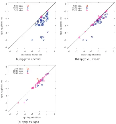
Figure 8 depicts the comparison ofnpqrperformance with each ofuncond,linearandrqss

models. Each of three plots contain 60 points corresponding to 60 trials (3 differentτs times 20 data sets).9 The vertical axis indicates the log pinball losses ofnpqr and the horizontal axis indicates those of the alternative. The points under (over) the 45 degree line means that the npqr was better (worse) than the alternative. Circles (squares) indicate that npqr was significantly better (worse) than the alternative at 0.05 significance level in paired-sample

t-test, while triangles indicate no significant difference.

• In terms of ramp loss (quantile property), the performance of ournpqrwere comparable to other three models for intermediate quantile (τ=0.5). All four models produced ramp losses close to the desired quantile, although flexible nonparametric modelsrqss andnpqr were noisier in this regard. Whenτ=0.5, the number of fτ(x) which exceed y did NOT deviate significantly from the binomial distribution B(sample size,τ)in all 20 data sets.

On the other hand, for extreme quantiles (τ=0.1 and 0.9),rqss andnpqr showed a small but significant bias towards the median in a few trials. We conjecture that this bias is related to the problem of data piling (Hall et al., 2005). See section 6 for the discussion.

Note that the quantile property, as such, is not informative measure for conditional quantile estimation. It merely measures unconditional quantile estimation performances. For example,

uncond, the constant function based on the unconditional quantile estimator with respect to

Y (straightforwardly obtained by sorting_{yi}m_i=1without using{xi}m_i=1at all), performed best

under this criterion. It is clear that the less flexible model would have the better quantile property, but it does not necessarily mean that those less flexible ones are better for conditional quantile functions.

-6 -5 -4 -3 -2 -1 0

-6 -5 -4 -3 -2 -1 0

npqr log pinball loss

uncond log pinball loss 0/60 trials

53/60 trials 7/60 trials

-6 -5 -4 -3 -2 -1 0

-6 -5 -4 -3 -2 -1 0

npqr log pinball loss

linear log pinball loss 0/60 trials

33/60 trials 27/60 trials

(a)npqrvsuncond (b)npqrvslinear

-6 -5 -4 -3 -2 -1 0

-6 -5 -4 -3 -2 -1 0

npqr log pinball loss

rqss log pinball loss 2/48 trials

10/48 trials 36/48 trials

(c)npqrvsrqss

Figure 8: Log-log plots of out-of-sample performances. The plots shownpqrversus (a)uncond,

(b)linearand (c)rqss; combining the average pinball losses of all 60 trials (3 quantiles

5.2 Experiments on Nonparametric Quantile Regression with Additional Constraints

We empirically investigate the performances of nonparametric quantile regression estimator with the additional constraints described in section 3. Imposing constraints is one way to introduce the prior knowledge on the data set being analyzed. Although additional constraints always increase training errors, we will see that these constraints can sometimes reduce test errors. The full results are shown in Appendix B.

5.2.1 NON-CROSSINGCONSTRAINTS

First we look at the effect of non-crossing constraints on the generalization performances. We used the same 20 data sets mentioned in the previous subsection. We denote the npqrs trained with non-crossing constraints asnoncrossandnpqrindicates standard one here. We made comparisons betweennpqrandnoncrosswithτ_{∈ {}0.1,0.5,0.9_}. The results fornoncrosswithτ=0.1 were obtained by training a pair of non-crossing models withτ=0.1 and 0.2. The results withτ=0.5 were obtained by training three non-crossing models with τ=0.4, 0.5 and 0.6. The results with τ=0.9 were obtained by training a pair of non-crossing models with τ=0.8 and 0.9. In this experiment, we simply impose non-crossing constraints only at a single test point to be evaluated. The kernel width and smoothing parameter were always set to be the selected ones in the above standardnpqrexperiments. The confidences were assessed by 10-fold cross-validation in the same way as the previous section. The complete results are found in the tables in Appendix B. The performances ofnpqrandnoncrossare quite similar sincenpqritself could produce almost non-crossing estimates and the constraints only make a small adjustments only when there happen to be the violations.

5.2.2 MONOTONICITYCONSTRAINTS

We compare two models:

• Nonparametric QR as described in Section 2 (npqr).

• Nonparametric QR with monotonicity constraints as described in Section 3.2 (npqrm).

We use two data sets:

• The cars data set as described in Mammen et al. (2001). Fuel efficiency (in miles per gallon) is studied as a function of engine output.

• The onions data set as described in Ruppert and Carroll (2003). log(Yield) is studied as a function of density, we use only the measurements taken at Purnong Landing.

We tested the performance of the two methods on 3 different quantiles (τ_{∈ {}0.1,0.5,0.9_}). In the experiments with cars, we noticed that the data is not truly monotonic. This is because, smaller en-gines may correspond to cheap cars and thus may not be very efficient. Monotonic models (npqrm) tend to do worse than standard models (npqr) for lower quantiles. With higher quantiles, npqrm

tends to do better than the standardnpqr. For theonionsdata set, as the data is truly monotonic,

6. Discussion and Extensions

Frequently in the literature of regression, including quantile regression, we encounter the term “ex-ploratory data analysis”. This is meant to describe a phase before the user has settled on a “model”, after which some statistical tests are performed, justifying the choice of the model. Quantile re-gression, which allows the user to highlight many aspects of the distribution, is indeed a useful tool for this type of analysis. We also note that no attempts at statistical modeling beyond automatic parameter choice via cross-validation, were made to tune the results. So the effort here stays true to that spirit, yet may provide useful estimates immediately.

In the Machine Learning literature the emphasis is more on short circuiting the modeling pro-cess. Here the two approaches are complementary. While not completely model-free, the experience of building the models in this paper shows how easy it is to estimate the quantities of interest in QR, with little of the angst of model selection, thanks to regularization. It is interesting to consider whether kernel methods, with regularization, can blur the distinction between model building and data exploration in statistics.

In summary, we have presented a Quadratic Programming method for estimating quantiles which bests the state of the art in statistics. It is easy to implement, comes with uniform con-vergence results and experimental evidence for its soundness. We also introduce non-crossing and monotonicity constraints as extensions to avoid some undesirable behaviors in some circumstances.

Overly Optimistic Estimates for Ramp Loss The experiments show us that the there is a bias towards the median in terms of the ramp loss. For example, if we run a quantile estimator with τ=0.05, then we will not necessarily get the empirical quantile is also at 0.05 but more likely to be at 0.08 or higher. Likewise, the empirical quantile will be 0.93 or lower if the estimator is run at 0.9. This affects all estimators, using the pinball loss as the loss function, not just the kernel version.

This is because the algorithm tends to aggressively push a number of points to the kink in the training set, these points may then be miscounted (see Lemma 3). The main reason behind it is that the extreme quantiles tend to be less smooth, the regularizer will therefore makes sure we get a simpler model by biasing towards the median (which is usually simpler). However, in the test set it is very unlikely to get the points lying exactly at the kink. Figure 9 shows us there is a linear relationship between the fraction of points at and below the kink (for low quantiles) and below the kink (for higher quantiles) with the empirical ramp loss.

Accordingly, in order to get a better performance in terms of the ramp loss, we just estimate the quantiles, and if they turn out to be too optimistic on the training set, we use a slightly lower (for τ<0.5) or higher (forτ>0.5) value ofτuntil we have exactly the right quantity.

The fact that there is a number of points sitting exactly on the kink (quantile regression - this paper), the edge of the tube (ν-SVR - see Sch¨olkopf et al., 2000), or the supporting hyperplane (single-class problems and novelty detection - see Sch¨olkopf et al., 1999) might affect the overall accuracy control in the test set. This issue deserves further scrutiny.

0 0.1 0.2 0.3 0.4 0.5 0.6 0.7

ram p loss 0.1

0.15 0.2 0.25

fr a c t io n o fp o i n ts a t a n d be lo w t he ki n k 1 . 0 = τ

0 0.2 0.4 0.6 0.8 1

ram p loss 0.4

0.5 0.6 0.7 0.8 0.9

1 fr a c tio n o fp o i n ts be lo w t he k i n k 9 . 0 = τ

Figure 9: Illustration of the relationship between quantile in training and ramp loss.

• Bivariate extreme-value distributions. Hall and Tajvidi (2000) propose methods to estimate

the dependence function of a bivariate extreme-value distribution. They require to estimate a convex function f such that f(0) =f(1) =1 and f(x)_≥max(x,1₋x)for x_∈[0,1]. We can also apply this approach to our method as to the monotonicity constraint, all we have to do is to ensure_hφ(0),w_i+b=_hφ(1),w_i+b=1,_hφ′′(x),w_{i ≥}0 and_hφ(x),w_i+b_≥max(x,1₋x) for x_∈[0,1].

• Positivity constraints. The regression function is positive. In this case, we must ensure

hφ(x),w_i+b>0,_∀x.

• Boundary conditions. The regression function is defined in[a,b]and assumed to be v at the

boundary point a or b.

• Additive models with monotone components. The regression function f :Rn→Ris of additive

form f(x1, ...,xn) = f1(x1) +...+fn(xn)where each additive component fiis monotonic.

• Observed deriatives. Assume that m samples are observed corresponding with m regression

functions. Now, the constraint is that fj coincides with the derivative of fj−1(same notation with last point) (Cox, 1988).

Future Work Quantile regression has been mainly used as a data analysis tool to assess the influ-ence of individual variables. This is an area where we expect that nonparametric estimates will lead to better performance.

Being able to estimate an upper bound on a random variable y_|x which hold with probabilityτ

Acknowledgments

National ICT Australia is funded through the Australian Government’s Backing Australia’s Ability initiative, in part through the Australian Research Council. This work was supported by grants of the ARC, by the Pascal Network of Excellence and by Japanese Grants-in-Aid for Scientific Research 16700258. We thank Roger Koenker for providing us with the latest version of the R packagequantreg, and for technical advice. We thank Shahar Mendelson and Bob Williamson for useful discussions and suggestions. We also thank the anonymous reviewers for valuable feedback.

Appendix A. Nonparametricν-Support Vector Regression

In this section we explore an alternative to the quantile regression framework proposed in Section 2. It derives from Sch¨olkopf et al. (2000). There the authors suggest a method for adapting SV regres-sion and classification estimates such that automatically only a quantileνlies beyond the desired confidence region. In particular, if p(y_|x) can be modeled by additive noise of equal degree (i.e.

y= f(x) +ξwhereξis a random variable independent of x) Sch¨olkopf et al. (2000) show that the ν-SV regression estimate does converge to a quantile estimate.

A.1 Heteroscedastic Regression

Whenever the above assumption on p(y|x) is violated ν-SVR will not perform as desired. This problem can be amended as follows: one needs to turn the marginε(x)into a nonparametric estimate itself. This means that we solve the following optimization problem.

minimize

θ1,θ2,b,ε

λ1 2kθ1k

2₊λ2 2kθ2k

2₊

∑

i=1

(ξi+ξ∗i)−νmε (30a)

subject to _hφ1(xi),θ1i+b−yi≤ε+hφ2(xi),θ2i+ξi (30b)

yi− hφ1(xi),θ1i −b≤ε+hφ2(xi),θ2i+ξ∗i (30c)

ξi,ξ∗i ≥0 (30d)

Hereφ1,φ2are feature maps,θ1,θ2are corresponding parameters,ξi,ξ∗i are slack variables and b,ε

are scalars. The key difference to the heteroscedastic estimation problem described in Sch¨olkopf et al. (2000) is that in the latter the authors assume that the specific form of the noise is known. In (30) instead, we make no such assumption and instead we estimateε(x)as_hφ2(x),θ2i+ε.

One may check that the dual of (30) is obtained by

minimize

α,α∗

1 2λ1

(α₋α∗)⊤K1(α₋α∗) + 1 2λ2

(α+α∗)⊤K1(α+α∗) + (α₋α∗)⊤y (31a)

subject to ~1⊤(α₋α∗) =0 (31b)

~₁⊤_(α+α∗_{) =Cmν (31c)}

0_≤αi,α∗i ≤1 for all 1≤i≤m (31d)

Here K1,K2are kernel matrices where[Ki]jl=ki(xj,xl)and~1 denotes the vector of ones. Moreover,

we have the usual kernel expansion, this time for the regression f(x)and the marginε(x)via

f(x) =

m

∑

i=1

(αi−α∗i)k1(xi,x) +b andε(x) =

m

∑

i=1

The scalars b andεcan be computed conveniently as dual variables of (31) when solving the problem with an interior point code (see Sch¨olkopf and Smola, 2002, for more details).

A.2 Theν-Property

As in the parametric case also (30) has theν-property. However, it is worth noting that the solution ε(x)need not be positive throughout unless we change the optimization problem slightly by impos-ing a nonnegativity constraint onε. The following theorem makes this reasoning more precise:

Theorem 8 The minimizer of (30) satisfies

1. The fraction of points for which_|yi−f(xi)|<ε(xi)is bounded by 1−ν.

2. The fraction of constraints (30b) and (30c) withξi>0 orξ∗i >0 is bounded from above byν.

3. If (x,y) is drawn iid from a distribution Pr(x,y), with Pr(y_|x) continuous and the

expecta-tion of the modulus of absolute continuity of its density satisfying lim_δ→0E[ε(δ)] =0. With

probability 1, asymptotically, the fraction of points satisfying_|yi−f(xi)|=ε(xi)converges to

0.

Moreover, imposingε_≥0 is equivalent to relaxing (31c) to~1⊤(α₋α∗_{)≤Cmν. If in addition K2}

has only nonnegative entries then alsoε(x)_≥0 for all xi.

Proof The proof is essentially similar to that of Lemma 3 and Sch¨olkopf et al. (2000). However note that the flexibility inε and potential ε(x)<0 lead to additional complications. However, if both f andε(x)have well behaved entropy numbers, then also f±εare well behaved.

To see the last set of claims note that the constraint~1⊤(α₋α∗_{)≤Cmνis obtained again directly}

from dualization via the conditionε_≥0. Sinceαi,α∗i ≥0 for all i it follows thatε(x)contains only

nonnegative coefficients, which proves the last part of the claim.

Note that in principle we could enforceε(xi)≥0 for all xi. This way, however, we would lose the

ν-property and add even more complication to the optimization problem. A third set of Lagrange multipliers would have to be added to the optimization problem.

A.3 An Example

The above derivation begs the question why one should not use (31) instead of (6) for the purpose of quantile regression. After all, both estimators yield an estimate for the upper and lower quantiles. Firstly, the combined approach is numerically more costly as it requires optimization over twice the number of parameters, albeit at the distinct advantage of a sparse solution, whereas (6) always leads to a dense solution.

The key difference, however, is that (31) is prone to producing estimates where the margin ε(x)<0. While such a solution is clearly unreasonable, it occurs whenever the margin is rather small and the overall tradeoff of simple f vs. simple εyields an advantage by keeping f simple. With enough data this effect vanishes, however, it occurs quite frequently, even with supposedly distant quantiles, as can be seen in Figure 10.

0 0.2 0.4 0.6 0.8 1

4

2

0

2

4

6

8

trainingdata supportvectors realmean

e

s

timated mean upp

erbar

l

ow erbar

0 0.2 0.4 0.6 0.8 1

!5

0

5

10

trainingdata supportvectors realm ean

e

s

timated mean upp

erbar lo

w

erbar

Figure 10: Illustration of the heteroscedastic SVM regression on artificial data set generated from (1) with f(x) =sinπx andσ(x) =exp(sin 2πx). On the left,λ1=1,λ2=10 andν=0.2, the algorithm successfully regresses the data. On the right,λ1=1,λ2=0.1 andν=0.2, the algorithm fails to regress the data asεbecomes negative.

the 0.05 quantile on the way. In addition to that, we make the assumption that the additive noise is symmetric.

We produced this derivation and experiments mainly to make the point that the adaptive margin approach of Sch¨olkopf et al. (2000) is insufficient to address the problems posed by quantile regres-sion. We found empirically that it is much easier to adjust QR instead of the symmetric variant.

In summary, the symmetric approach is probably useful only for parametric estimates where the number of parameters is small and where the expansion coefficients ensure thatε(x)_≥0 for all x.

Appendix B. Experimental Results

In this appendix, we show the detail results on the experiments.

B.1 Standard Nonparametric Quantile Regression

Here we assemble six tables to display the comparisons among four models,uncond,linear,rqss

andnpqr. Each table represents pinball loss or ramp loss for each ofτ=0.1, 0.5 and 0.9 cases. τ=0.1 τ=0.5 τ=0.9

Pinball Loss Table 2 Table 4 Table 6 Ramp Loss Table 3 Table 5 Table 7

Tables 2, 4, and 6 show the average pinball loss for each data set. A lower figure is preferred in each case. The bold figures indicate the best (smallest) performances. The circles ’_◦’ indicate that the difference from the second best model were statistically significant at 0.05 level with two-sided paired-sample t-test. NA denotes cases where rqss (Koenker et al., 1994) was unable to produce estimates, due to its construction of the function system.