Behavioral Shaping for Geometric Concepts
Manu Chhabra [email protected]
Department of Computer Science University of Rochester
Rochester, NY 14627, USA
Robert A. Jacobs [email protected]
Department of Brain and Cognitive Sciences University of Rochester
Rochester, NY 14627, USA
Daniel ˇStefankoviˇc [email protected]
Department of Computer Science University of Rochester
Rochester, NY 14627, USA
Editor: Manfred K. Warmuth
Abstract
In a search problem, an agent uses the membership oracle of a target concept to find a positive ex-ample of the concept. In a shaped search problem the agent is aided by a sequence of increasingly restrictive concepts leading to the target concept (analogous to behavioral shaping). The concepts are given by membership oracles, and the agent has to find a positive example of the target concept while minimizing the total number of oracle queries. We show that for the concept class of intervals on the real line an agent using a bounded number of queries per oracle exists. In contrast, for the concept class of unions of two intervals on the real line no agent with a bounded number of queries per oracle exists. We then investigate the (amortized) number of queries per oracle needed for the shaped search problem over other concept classes. We explore the following methods to obtain efficient agents. For axis-parallel rectangles we use a bootstrapping technique to obtain gradually better approximations of the target concept. We show that given rectangles R⊆A⊆Rdone can obtain a rectangle A0⊇R with vol(A0)/vol(R)≤2, using only O(d·vol(A)/vol(R))random sam-ples from A. For ellipsoids of bounded eccentricity inRdwe analyze a deterministic ray-shooting process which uses a sequence of rays to get close to the centroid. Finally, we use algorithms for generating random points in convex bodies (Dyer et al., 1991; Kannan et al., 1997) to give a randomized agent for the concept class of convex bodies. In the final section, we explore connec-tions between our bootstrapping method and active learning. Specifically, we use the bootstrapping technique for axis-parallel rectangles to active learn axis-parallel rectangles under the uniform dis-tribution in O(d ln(1/ε))labeled samples.
Keywords: computational learning theory, behavioral shaping, active learning
1. Introduction
training procedure commonly used to teach complex behaviors. Using this procedure, a complex task is taught to a learner in an incremental manner. The learner is initially rewarded for performing an easy task that coarsely resembles the target task that the teacher wants the learner to perform. Over time, the learner is rewarded for performing more difficult tasks that monotonically provide better approximations to the target task. At the end of the training sequence, the learner is rewarded only for performing the target task. Shaping was first proposed by B. F. Skinner in the 1930s (Skinner, 1938). In addition to training humans and other organisms, behavioral shaping has also been used in artificial intelligence applications such as those that arise in robotics or reinforcement learning (Dorigo and Colombetti, 1994; Mataric, 1994; Randløv and Alstrøm, 1998; Konidaris and Barto, 2006; Ng et al., 1999).
The goal of this paper is to mathematically formalize the notion of shaping, and to show that shaping makes certain tasks easier to learn. We specifically study shaping in the context of search problems (for a learning theoretic analysis of a similar search problem, see, e.g., Fine and Mansour, 2006). In a search problem, the task is to find one positive example of a concept given a membership oracle of the concept using as few queries to the oracle as possible. If a shaping sequence, which is a sequence of nested concepts, is available, it might be possible to solve the search problem with a smaller number of oracle queries. When concepts are standard geometrical concepts like rectangles, balls, ellipsoids, and convex bodies in high dimensions, we show efficient algorithms to solve the search problem using a shaping sequence.
“Reward shaping” of Ng et al. (1999) and quasi-convex optimization are related to our work. Ng et al. (1999) gave conditions under which “reward shaping” works in a reinforcement learning setting. In their framework, shaping is a transformation of the reward function and the goal is to formalize conditions under which this transformation preserves value of the underlying policies. Our framework is different from Ng et al. (1999) in at least two ways. First, we have a sequence of reward functions as compared to their one step reward transform. Second, our reward functions are binary whereas they allow general, real valued rewards.
A weaker version of the shaped search problem in which the concepts are convex and all the oracles are available to the agent simultaneously can be viewed as an instance of a quasi-convex optimization problem. Also, we cannot apply the algorithms from this area since they usually rely on an oracle (so called separation oracle) stronger than the membership oracle that we use. What makes our setting different is that the oracles are available in a fixed order, and we only have membership oracles. Our framework is motivated by behavioral shaping (Skinner, 1938), as well as practical robotics (Dorigo and Colombetti, 1994).
Our work is similar in spirit to the idea of using a helpful teacher (Goldman and Kearns, 1991; Goldman et al., 1993; Goldman and Mathias, 1993; Heged ˝us, 1994). For example, Goldman and Kearns (1991) considered a model where a helpful teacher chose examples to allow a learner to uniquely identify any concept in a given concept class. Our model differs from Goldman and Kearns (1991) in the following aspects. First, the teacher in Goldman and Kearns (1991) is “active” (it is directly providing the learner with “good” examples), whereas in our model the burden of choosing good queries is on the learner. Second, the learner in Goldman and Kearns (1991) is faced with a more general task of identifying the concept, whereas our learner is solving a search problem.
explains and analyzes the center-point algorithm which is used in Section 6 to solve the shaped search problem for bounded eccentricity ellipsoids. Section 7 uses the techniques on sampling random points from a convex body to solve the problem for general convex bodies. In Section 8 we define the problem of one-sided active learning, and show that the bootstrapping algorithm given in Section 4 can be used to active-learn the concept class of axis-parallel rectangles with
O(d ln(1/ε))labeled samples. Finally, Section 9 wraps up the paper with a discussion and possible future directions.
2. A Formal Model of Behavioral Shaping
A search problem is defined by a pair of sets(S,T)such that T ⊆S (S is the starting set and T is
the target set). A search agent “knows” S and has to find a point y∈T . The set T will be given by a
membership oracle. The goal of the agent is to minimize the number of queries to the oracle. Of course without any conditions on (S,T) the agent could be searching for a needle in a haystack and require an unbounded number of queries. To make the problem reasonable we will as-sume that S and T come from some concept class
C
(e. g., S,T could be intervals inR), and that the volume vol(T)is not too small compared to the volume vol(S)(i. e., T is not a needle in a haystackS).
Before formally defining a search problem we need the following standard notions from learning theory (see, e.g., Anthony and Biggs, 1992; Kearns and Vazirani, 1994). Let(X,
B
)be a measurable space and let vol be a measure on(X,B
). LetC
⊆B
. The setC
is called a concept class and its members are called concepts. We will assume thatC
comes with a representation scheme (see Kearns and Vazirani, 1994, Chapter 2). Examples of concept classes that we study include intervals inR, axis-parallel rectangles inRd, ellipsoids inRd, and convex bodies inRd. We will restrict our attention to the Lebesgue measure onRd.Definition 2.1 Let
C
be a concept class. A search problem is defined by a pair of concepts(S,T)such that T⊆S and S,T ∈
C
. The agent has a representation of S and has to find a point in T using a membership oracle for T .Note that for any concept class there is a natural “oblivious” randomized algorithm for the search problem: query independent uniform random points from S until you find a point in T . The expected number of queries of the algorithm is vol(S)/vol(T). For sufficiently complicated concept classes (e. g., finite unions of intervals) the use of randomness might be inevitable—a deterministic algorithm with bounded number of queries need not exist (the question of deterministic search is related to the concept of hitting sets, see, e.g., Linial et al., 1993).
For concept classes we will consider one can find Ω(n) disjoint concepts, each of volume Ω(1/n). The following observation implies that the trivial algorithm is the best possible (up to a constant factor).
Observation 2.1 Suppose that there exist disjoint concepts T1, . . . ,Tn⊆S. Let i be uniformly
ran-dom from [n]. The expected (over the choice of i) number of queries made by any (randomized) agent on(S,Ti)isΩ(n).
shrinking concepts from the underlying concept class
C
. The rate of shrinking will be controlled by a parameter, denotedγ.Definition 2.2 Letγ∈(0,1). Let
C
be a concept class and let(S,T)be a search problem overC
. A sequence of concepts S0⊇S1⊇ ··· ⊇Sk is called aγ-shaping sequence if S0=S, Sk =T , and vol(St+1)≥γvol(St)for all t∈ {0, . . . ,k−1}.A search agent in a shaped search problem only has access to the membership oracles of
S1, . . . ,Sk. However, if the agent makes a query to St, it can no longer make a query to Sj with
j<t. In other words, the oracles St are presented to the agent in k iterations, with the agent making (zero or more) queries to the oracle St at iteration t. The agent successfully solves the shaped search problem if at the end of the process it outputs x∈T . We assume that the agent knows the value ofγ
and does not know the value of k. However, before the last iteration the agent is informed that it is accessing the last oracle.
We will evaluate the performance of the agent by the amortized number of membership queries per oracle (i. e., the total number of queries divided by k). We will also consider randomized agents, which are zero-error probability (Las Vegas) algorithms (i. e., they are always successful). For a randomized agent the performance is measured by the expected number of membership queries per oracle, where the expectation is taken over the coin flips of the agent. This is formalized in the following definition.
Definition 2.3 Let
C
be a concept class. LetA
be a search agent. We say that the agentA
solvesa γ-shaped search problem using q queries per oracle, if for every S,T ∈
C
, every k, and everyγ-shaping sequence S0, . . . ,Sk∈
C
the total number of queries made by the agent is bounded by kq. If the agent is randomized we require the expected total number of queries to be bounded by kq.Note that forγ>γ0anyγ-shaping sequence is aγ0-shaping sequence. Thus asγ→1 the shaped search problem becomes easier. We will study howγaffects the complexity of the shaped search problem.
2.1 Our Results
In order to introduce the shaped search problem, we start with a positive and a negative result for two simple concept classes (the proofs are in Section 3). First, we show that O(1/γ) queries per oracle suffice to solve theγ-shaped search problem for the concept class of closed intervals inR.
Proposition 2.4 Let
C
be the concept class of closed intervals in R. There exists a deterministic agent which for anyγuses O(1/γ)queries per oracle to solveγ-shaped search problem.Next, we contrast the Proposition 2.4 by showing that for the class of “unions of two closed intervals inR” there exists no agent that solves theγ-shaped search problem using bounded number of queries per oracle.
Proposition 2.5 Let
C
be the concept class of unions of two closed intervals inR. Letγ∈(0,1). For every (randomized) agentA
and every number q there exists a search problem(S,T), k, and aWe understand the concept class of intervals completely as Proposition 2.4 can be strengthened as follows.
Proposition 2.6 Let
C
be the concept class of closed intervals inR. Let f(γ) =1/γforγ≤1/2,and f(γ) =ln(1/γ) forγ>1/2. There exists a deterministic agent which for anyγ∈(0,1) uses O(f(γ))queries per oracle to solveγ-shaped search problem. On the other hand, for anyγ∈(0,1), any (randomized) agent makes at leastΩ(f(γ))queries per oracle.
The shaped search problem for axis-parallel rectangles inRd turns out to be more complicated. Here we do not understand the dependence of the complexity of theγ-shaped search problem onγ. We present three algorithms; each algorithm works better than the other two for a certain range of γ.
We say that a randomized agent is oblivious if for every oracle St the queries to St which lie in
St are independent and uniformly random in St.
Theorem 2.7 Let
C
be the concept class of axis-parallel rectangles inRd.1. For anyγthere exists a randomized agent using O(1γ+ (d+ln1γ)ln d)queries per oracle. 2. For anyγthere exists an (oblivious) randomized agent using O(d/γ)queries per oracle.
3. For any constantγ>1/2 there exists a deterministic agent using O(ln d)queries per oracle.
The following table compares the number of queries used by the algorithms for various values ofγ.
Alg. 1. Alg. 2. Alg. 3. γ=3/4 O(d ln d) O(d) O(ln d)
γ=1/4 O(d ln d) O(d) N/A γ=1/ln d O(d ln d) O(d ln d) N/A γ=1/d O(d ln d) O(d2) N/A
Note that the deterministic algorithm for part 3. uses less queries than the randomized algorithm for part 2., but it only works in a very restricted range ofγ. It relies on the following fact: the centroid of an axis-parallel rectangle of volume 1 is contained in every axis-parallel sub-rectangle of volume
≥1/2. It would be interesting to know whether the logarithmic dependence on d could be extended for constantsγ≤1/2, or, perhaps, a lower bound could be shown.
Question 1 AreΩ(d)queries per oracle needed forγ<1/2?
The simple agent for the part 1) of Theorem 2.7 is described in Section 3.
In Section 4 we introduce the concept of “bootstrap-learning algorithm”. A bootstrap-learning algorithm, given an approximation A1of an unknown concept C∈
C
and a membership oracle forC, outputs a better approximation A2 of C. We show an efficient bootstrap-learning algorithm for the concept class of axis-parallel rectangles and use it to prove part 2) of Theorem 2.7.
Part 3) of Theorem 2.7 is proved in Section 5. We show how an approximate center of an axis-parallel rectangle can be maintained using only O(ln d)(amortized) queries per oracle. Ifγis not too small, the center of St will remain inside St+1and can be “recalibrated”.
following process can be used to get close to a centroid of K: pick a line `through the current point, move the current point to the center of`∩K and repeat. If`is uniformly random the process converges to the centroid of K. It would be interesting to know what parameters influence the convergence rate of this process.
Question 2 How many iterations of the random ray-shooting are needed to getε-close to the cen-troid of a (isotropic), centrally symmetric convex body K?
We will consider the following deterministic version of the ray-shooting approach: shoot the rays in the axis directions e1, . . . ,ed, in a round-robin fashion.
Question 3 How many iterations of the deterministic round-robin ray-shooting are needed to get ε-close to the centroid of a (isotropic), centrally symmetric convex body K?
In Section 6 we study a variant of the deterministic ray-shooting which moves to a weighted average of the current point and the center of K∩`. We analyze the process for the class of ellipsoids of bounded eccentricity. As a consequence we obtain:
Theorem 2.8 Let
C
be the concept class of ellipsoids with eccentricity bounded by L. Letγ>1/2.Theγ-shaped search problem can be solved by a deterministic agent using O(L2·d3/2ln d)queries
per ray-shooting oracle (a ray-shooting oracle returns the points of intersection of K with a line through a point x∈K)
The requirementγ>1/2 in Theorem 2.8 can be relaxed. Similarly, as in the axis-parallel rect-angle case, we need a condition on the volume of a sub-ellipsoid of an ellipsoid E which guarantees that the sub-ellipsoid contains the centroid of E. We do not determine this condition (which is a function of L and d).
To prove Theorem 2.8 we need the following interesting technical result.
Lemma 2.9 Let v1, . . . ,vd∈Rd be orthogonal vectors. Letα∈(0,2)and L≥1. Let D be an d×d
diagonal matrix with diagonal entries from the interval[1/L,1]. Let
M(α) = n
∏
i=1
I−α·Dviv
T iD
vT iD2vi
.
Then
kM(1/√d)k22≤1− 1 5L2√d.
Using random walks and approximating ellipsoids (Bertsimas and Vempala, 2004; Kannan et al., 1997; Gr¨otschel et al., 1988; Lov´asz, 1986) we can show that convexity makes the shaped search problem solvable. We obtain the following result (a sketch of the proof is in Section 7):
Theorem 2.10 Let
C
be the concept class of compact convex bodies in Rd. For any γ∈(0,1)3. Basic Results for Intervals and Axis-parallel Rectangles
Now we show that for intervals O(1/γ)queries per oracle are sufficient to solve theγ-shaped search problem. For each St we will compute an interval[at,bt]containing St such that the length of[at,bt] is at most three times longer than the length of St. By querying St+1 on a uniform set of O(1/γ) points in[at,bt]we will obtain[at+1,bt+1].
Proof of Proposition 2.4:
The agent will compute an interval approximating St for t=0, . . . ,k. More precisely it will compute
at and bt such that St ⊆[at,bt]and vol(St)≥(bt−at)/3. Initially we have S=S0=:[a0,b0]and vol(S0) = (b0−a0)≥(b0−a0)/3.
Suppose that St ⊆[at,bt]and vol(St)≥(bt−at)/3. Using an affine transformation we can, w.l.o.g., assume at =0 and bt =1. Thus vol(St)≥1/3 and vol(St+1)≥γ/3.
Let Q0={0,1}, Q1={0,1/2,1}, . . . , Qi={j/2i|j=0, . . . ,2i}. The agent will query St+1on all points in Qi, i=0,1, . . ., until it finds the smallest j such that|Qj∩St+1| ≥2. Choose at+1and
bt+1such that
Qj∩St+1={at+1+2−j, . . . ,bt+1−2−j}.
For this at+1,bt+1we have St+1⊆[at+1,bt+1]and vol(St+1)≥(bt+1−at+1)/3.
Note that if 2−i≤γ/6 then|Ai∩St+1| ≥2. By the minimality of j we have 2j≤12/γand hence the total number of queries per oracle is O(1/γ).
Proof of Proposition 2.6:
First we show the upper bound of O(ln(1/γ))forγ>1/2. Let`=d−ln 2
lnγe. Note thatγ
`≥1/4. Now
we use the agent from Proposition 2.4 on oracles S0,S`,S2`, . . ., and we do not query the rest of the oracles at all. The number of queries per oracle is O(1/`) =O(ln(1/γ)).
Next we show the lower bound of Ω(1/γ)forγ<1/2. We take a shaping sequence of length
k=1. Note that there existb1/γcdisjoint intervals of lengthγin[0,1]and hence, by Observation 2.1, the agent needs to makeΩ(b1/γc)queries (per oracle).
Finally, the lower bound ofΩ(ln(1/γ))will follow by an information-theoretic argument. As-sume that the agent is deterministic. Fix an integer k. There exist Ω(1/γk) disjoint intervals of lengthγk. For each of these intervals there exists a shaping sequence of length k ending with that interval. We will randomly pick one of these shaping sequences and present it to the agent. The agent, using Q queries, identifies which interval (out of theΩ(1/γk)intervals) we chose. This im-plies E[Q] =Ω(k ln(1/γ)), and hence the number of queries per oracle isΩ(ln(1/γ)). The lower bound for a randomized agent follows by Yao’s min-max lemma (see, e.g., Motwani and Raghavan,
1995, Chapter 2).
For unions of two intervals the agent can be forced to make many queries per oracle. If one of the intervals is large and one is small then the small interval can abruptly shrink. We will use this to “hide” the target T . Then we will shrink the large interval until it disappears. Now the agent is forced to find the hidden target T , which requires a large number of queries.
Proof of Proposition 2.5:
γ-shaping sequence will be the following:
St =
( [−1,0]∪[0,γt] for t=0, . . . ,n,
[−γt−n−1,0]∪T for t=n+1, . . . ,3n+`+1,
T for t=3n+`+2.
Note that St is always a union of two intervals. In the first n+1 iterations, the right hand-side interval is shrinking. When the right-hand side interval is sufficiently small we can replace it by the “hidden” interval T . After that we shrink the left-hand side until we make it disappear.
For the sake of the lower bound argument, we will help the agent by telling it the general shape of the shaping sequence, but we will keep the location of T secret. Now, w.l.o.g, we can assume that the agent only queries points in[0,γn]on the oracle for T (because for all the other queries the agent can figure the answer himself). By Observation 2.1 the agent needsΩ(1/γ`)queries to find a point in T . Hence the number of queries per oracle is
Ω 1/γ`
3n+`+2
.
Letting`→∞we obtain that the number of queries per oracle is unbounded.
Now we describe an agent for axis-parallel rectangles. Let At be a tight rectangle containing
St (i. e., a rectangle such that vol(At)≤C·vol(St)for some constant C). We will sample random points in At until we get a point y inside St+1. Then we will shoot rays from y in the axis-parallel directions to find the approximate boundary of St+1. From this we will obtain a tight rectangle At+1 containing St+1.
Proof of the part 1) of Theorem 2.7:
We will compute axis-parallel rectangles A0, . . . ,Ak such that St ⊆At and vol(At)≤e vol(St)(for
t=0, . . . ,k). Clearly we can take A0=S0.
Suppose that we have At such that St ⊆At, and vol(At)≤e vol(St). Using an affine trans-formation we can, w.l.o.g, assume At = [0,1]d. Since the St form aγ-shaping sequence we have vol(St+1)≥γ/e. We will sample random points from At, until we get a point x inside St+1. In expectation we will need to query at most e/γpoints to find x.
Now that we have x we will try to approximate St+1in each dimension separately. We will find the smallest j≥0 such that x+2−je1∈St+1, or x−2−je1∈St+1. Only O(−ln w1(St+1))queries are needed for this step (where w1(St+1)is the width of St+1in the 1-st dimension).
Then using binary search on [0,21−j] we will find y such that x+ye
1∈St+1 and x+ (y+ 2−j−1/d)e16∈St+1. This step uses only O(ln d) queries. Similarly we will find z∈[0,21−j]such that x−ze1∈St+1and x−(z+2−j−1/d)e16∈St+1. Note that
I1:= [x−(z+2−j−1/d),x+ (y+2−j−1/d)],
contains the projection of St+1 into the 1-st dimension, and the the length of I1 is at most (1+ 1/d)w1(S).
Analogously we compute the Iifor i=1, . . . ,d. The total number of queries is
O(d ln d) +O −
d
∑
i=1
ln w1(St+1)
!
=O
d ln d+ln1 γ
.
4. (α,β)-bootstrap Learning Algorithms
In this section we prove the part 2) of Theorem 2.7. We cast the proof in a general setting that we call “bootstrap-learning algorithms”.
Definition 4.1 Let
C
,C
Abe concept classes. Letα>β≥1. An(α,β)-bootstrap learning algorithmfor
C
usingC
A takes as an input a representation of a concept A1∈C
A and an oracle for a conceptR∈
C
. The concepts A1 and R are guaranteed to satisfy R⊆A1 and vol(A1)≤α·vol(R). The algorithm outputs a representation of a concept A2∈C
Asuch that R⊆A2and vol(A2)≤β·vol(R). The efficiency of the algorithm is measured by the worst-case (expected) number T of oracle queries to R (i. e., we take the worst A1and R fromC
).If an efficient(α,β)-bootstrap learning algorithm exists for a concept class
C
then it can be used for the shaped search problem as follows.Lemma 4.2 Let
C
,C
A be concept classes. Let α>β≥1. Assume that there exists an (α,β)-bootstrap learning algorithm for
C
usingC
A using T queries. Suppose that for every C∈C
thereexists A∈
C
A such that C⊆A and vol(A)≤β·vol(C). Then there exists an agent which for any γ≥β/αsolves theγ-shaped search problem (overC
) using T queries per oracle.Proof :
We will compute A0, . . . ,Ak ∈
C
A such that St ⊆At and vol(At)≤β·vol(St). By the assumption of the lemma the first A0 exists. (The starting concept S in a shaped search problem is known in advance and hence the agent can pre-compute A0.)Suppose that we have At. Then St+1⊆At, and vol(At)≤(β/γ)vol(St+1)≤αvol(St+1). Hence using the(α,β)boot-strap algorithm we can find At+1, using only T queries.
If one uses Lemma 4.2 to obtain an agent for the shaped search problem for
C
, one should chooseC
A which allows for an efficient(α,β)-bootstrap algorithm. Later in this section we will show that for axis-parallel rectangles one can takeC
A=C
, and obtain an efficient(α,β)-bootstrap algorithm. Are there concept classes for which it is advantageous to chooseC
A6=C
? More generally one can ask:Question 4 For given concept class
C
, and α>β≥1, which concept classesC
A allow for anefficient(α,β)-bootstrap learning algorithm?
input : a representation of A1∈CAand an oracle for R∈C assume : R⊆A1and vol(A1)≤α·vol(R).
output : a representation of A2∈CA, such that
R⊆A2and vol(A2)≤β·vol(R).
S+←/0, S−←/0 1
repeat 2
pick a random point p∈A1 3
if p∈R then S+←S+∪ {p}else S−←S−∪ {p}fi 4
PossibleR← {C∈C|S+⊆C⊆A1\S−} 5
v←the minimal volume of a concept in PossibleR 6
A2←a concept of minimal volume inCAcontaining all C∈PossibleR 7
until vol(A2)≤β·v 8
output a representation of A2 9
Algorithm 1: Inner-Outer algorithm for(α,β)-bootstrap learning
Note that the set PossibleR contains R and hence R⊆A2, and v ≤vol(R). Thus when the algorithm terminates we have vol(A2)≤β·v≤β·vol(R). Thus we have the following observation. Proposition 4.3 The Inner-Outer algorithm is an(α,β)-bootstrap learning algorithm.
Now we analyze the Inner-Outer algorithm for the concept class of axis-parallel rectangles with
C
A=C
. We will need the following technical results (the proofs are in the appendix).Lemma 4.4 Let X1, . . . ,Xnbe i.i.d. uniformly random in the interval[0,1]. Then
E
−ln
max
i Xi−mini Xi
= 2n−1
n(n−1) ≤
2
n−1 ≤ 4
n.
Lemma 4.5 Let K be from the binomial distribution B(n,p). Let X1, . . . ,XK be i.i.d. uniformly
random in the interval[0,1]. Then
E[min{1,X1, . . . ,XK}] =
1−(1−p)n+1 (n+1)p ≤
1
np.
Lemma 4.6 Let
C
be the set of axis-parallel rectangles inRd. LetC
A=C
. The expected numberof oracle calls made by the Inner-Outer algorithm is bounded by 8+320dα/lnβ.
As an immediate corollary we obtain:
Proof of the part 2) of Theorem 2.7:
Immediate from Lemma 4.6 and Lemma 4.2.
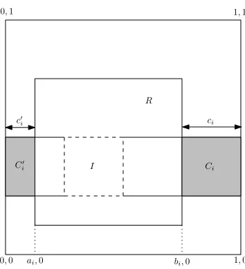
Proof of Lemma 4.6:
W.l.o.g. we can assume A1= [0,1]d. Let R= [a1,b1]× ··· ×[ad,bd], where 0≤ai≤bi≤1, for
i=1, . . . ,d.
I
0,0 1,0
1,1 0,1
R
C0
i Ci
ai,0 bi,0
ci c0
i
Figure 1: Schematic drawing for the proof of Lemma 4.6.
In the first phase n1 i.i.d. random points from A1 are sampled. The expected number of points that fall inside R is at least n1/α. By Chernoff bound with probability at least 3/4 we get at least
n1/(2α)points inside R. With probability at most 1/4 the algorithm “fails”.
From now on we assume that the algorithm did not “fail”, i. e., at least n1/(2α)points are inside
R. Let I be the smallest rectangle containing these points. We will choose n1>4αand hence, by Lemma 4.4, the expected logarithm of the width of I in the i-th dimension satisfies
E
−ln wi(I)
bi−ai
≤8αn
1
. (1)
Summing the (1) for i∈[d]we obtain (using the linearity of expectation)
E
lnvol(R) vol(I)
≤8dαn
1
. (2)
Markov inequality applied to (2) yields that with probability at least 3/4 we have
lnvol(R) vol(I) ≤
32dα
n1
. (3)
If (3) is not satisfied we say that the algorithm “failed”.
From now on we assume that (3) is true, i. e., the algorithm did not fail. Thus
vol(I)≥vol(R)·exp
−32dαn
1
. (4)
Now we sample n2 i.i.d. random points from A1. A point falls inside Ci with probability vol(Ci) =civol(I)/(bi−ai). The expected distance of the point in Ciclosest to R, by Lemma 4.5, is bounded by
ci·
1
n2·civol(I)/(bi−ai)
= bi−ai
n2vol(I)
. (5)
Note that A2 determined by the closest points in the Ci and Ci0 contains PossibleR. By (5) the expected width of A2 in the i-th dimension satisfies E[wi(A2)]≤(bi−ai)(1+2/(n2vol(I))). By Jensen’s inequality
E
lnwi(A2)
bi−ai
≤ln
1+ 2
n2vol(I)
≤ 2
n2vol(I) .
By the linearity of expectation
E
lnvol(A2) vol(R)
≤n 2d
2vol(I) .
By Markov inequality with probability at least 3/4 we have
lnvol(A2) vol(R) ≤
8d
n2vol(I) ≤ 8dα
n2
, (6)
and hence
vol(R)≥vol(A2)·exp
−8dαn
2
. (7)
Again, if (6) is false we say that the algorithm “failed”. Note that the algorithm “failed” (in any of the three possible ways) with probability at most 3/4. Thus with probability 1/4 we have that (4) and (7) are true and hence
vol(A2)≤vol(I)·exp
8dα
n2
+32dα
n1
.
For n1=d64dα/lnβe and n2=d16dα/lnβe the right hand side is bounded byβ and hence the algorithm will terminate.
Note that additional points in S+and S−do not “hurt” the algorithm (removal of a point cannot increase v, nor can it decrease vol(A2)). Thus if the algorithm does not terminate, the next run of length n1+n2 terminates with probability≥1/4, etc. Hence in expectation at most 4(n1+n2)
oracle queries suffice.
5. Center-point Algorithm
In this section we show how an approximate center-point of a rectangle can be maintained using only O(ln d)queries per oracle. As a corollary we obtain a proof of the part 3) of Theorem 2.7.
Given a vector v ∈Rd, let Piv be the projection of v to the i-th dimension (i. e., the vector obtained by zeroing out all the entries of v except the i-th coordinate). Let∂S denote the boundary
of the S.
Definition 5.1 Let S be an axis-parallel rectangle inRd. Letε∈(0,1). Let x be a point in S and let v∈Rd, v≥0. Letαi,βi≥0 be determined by x+αi(Piv)∈∂S and x−βi(Piv)∈∂S, for i∈[d]. We say that v is anε-approximate distance vector for(S,x)if 1−ε≤αi≤1 and 1−ε≤βi≤1 for
i∈[d]. We say that x is anε-approximate center-point of S if there exists anε-approximate distance
Note that if v is anε-approximate distance vector for(S,x)then we have
d
∏
i=1 (2vi)≥
d
∏
i=1
((αi+βi)vi) =vol(S). (8)
If S0⊆S and the volume of S0 is not much smaller than the volume of S then an approximate center-point x of S should be contained in S0. The next lemma formalizes this intuition.
Lemma 5.2 Let S0⊆S be axis-parallel rectangles. Assume that vol(S)/vol(S0)≤2−2ε. Let x∈ S be an ε-approximate center-point of S. Then x∈S0. Moreover, for α0i,β0i ≥0 determined by
x+α0
i(Piv)∈∂S0and x−β0i(Piv)∈∂S0we haveα0i+β0i≥1, andα0i≥ε/2, andβ0i≥ε/2.
Now we give an algorithm which “recalibrates” an ε-approximate center-point. Note that the first two steps of the algorithm rely on the fact that x∈S0(which is guaranteed by Lemma 5.2).
input : x∈S, and anε-approximate distance vector v for(S,x). assume : S0⊆S and vol(S)≤(2−2ε)vol(S0)
output : x0∈S0, and anε-approximate distance vector v0for(S0,x0). findδ+>0 such that x+ (δ++ε/8)v6∈S0and x+δ+v∈S0
1
findδ−>0 such that x−(δ−+ε/8)v6∈S0and x−δ−v∈S0 2
letδ=min{δ+,δ−}, let s= +1 ifδ=δ+and s=−1 otherwise 3
ifδ<1−εthen 4
find j∈[d]such that x+s(δ+ε/8)(Pjv)6∈S0and x+sδ(Pjv)∈S0 5
findα>0 such that x+ (α+ε/8)(Pjv)6∈S0, and x+α(Pjv)∈S0 6
findβ>0 such that x−(β+ε/8)(Pjv)6∈S0, and x−β(Pjv)∈S0 7
update xj←xj+vj(α−β)/2 8
update vj←(1+ε/4)((α+β)/2)vj 9
go to step 1 10
return x,v
11
Algorithm 2: Center-point algorithm
Proof of Lemma 5.2:
Let v be anε-approximate distance vector for(S,x). Suppose x6∈S0. Then there exists a coordinate
i∈[d] such that S0 lies on one side of the hyperplane {z ∈Rd|z
i=xi}. Thus the width of S0 in the i-th dimension satisfies wi(S0)≤vi. On the other hand wi(S)≥wi(S0) + (1−ε)vi. Hence
wi(S)/wi(S0)≥2−εwhich implies vol(S)/vol(S0)≥2−ε, a contradiction. We proved x∈S0. For any i∈[d], usingαi,βi≥1−ε, we obtain
2−2ε≥ vol(S) vol(S0) ≥
αi+βi α0
i+β0i
≥ α20−2ε
i+β0i ,
and henceα0i+β0 i≥1.
Similarly, for any i∈[d], usingβ0i≤βi≤1,α0i≤αi, we obtain
2−2ε≥ vol(S) vol(S0) ≥
αi+βi α0
i+β0i
≥ααi0+βi
i+βi ≥ αi+1 α0
i+1
≥α20−ε
i+1 .
This impliesα0i≥ε/2. The proof ofβ0i≥ε/2 is the same.
When|δ| ≥1−εon step 4 then x+ (1−ε)v∈S0and x−(1−ε)v∈S0, and hence theαiandβi are bounded by 1−εfrom below. Thus the final v isε-approximate distance vector for(S0,x).
It remains to show that during the algorithm theαiandβifor x,v,S0always remain bounded by 1 from above. Let x0j =xj+vj(α−β)/2 and v0j= (1+ε/4)((α+β)/2)vj, i. e., x0j and v0j are the new values assigned on lines 8 and 9. We have
x0j+v0j=xj+vj
α+ε(α+β)
8
≥xj+vj(α+ε/8), (9)
and
x0j+ (1−ε)v0j=xj+vj
α
−β
2 + (1+ε/4)(1−ε)
α+β
2
≤xj+αvj. (10)
From (9) and (10) and our choice ofαon line 6 it follows that on line 10 the value ofαj for the new
x and v satisfies 1−ε≤αj≤1. Similar argument establishes 1−ε≤βj≤1. Note that
v0j
vj
= (1+ε/4)α+β
2 ≤(1+ε/4)(1−ε/2)≤1−ε/4. (11)
We will use (11) to bound the amortized number of steps we spend in our application of the center-point algorithm.
Proof of the part 3) of Theorem 2.7:
W.l.o.g., assume S=S0= [0,1]d. Let x(0)=v(0)= (1/2, . . . ,1/2). Note that v(0)is anε-approximate distance vector for(S0,x(0)). We will use the center-point algorithm to compute x(t),v(t) such that
v(t)is anε-approximate distance vector for(St,x(t)).
Before we start analyzing the algorithm let us emphasize that we defined “queries per oracle” to be an “amortized” quantity (as opposed to a “worst-case” quantity). Thus it is fine if the algorithm makesΘ(d)queries going from St to St+1, as long as the average number of queries per oracle is
O(ln d).
Now we analyze the number of queries per oracle. Let
Φt =∏
d i=1(2v
(t) i ) vol(St)
.
Note thatΦ0=1, and, by (8),Φt≥1 for every t=0, . . . ,k.
From (11) it follows that every time the step on line 10 is executed, the value of Φt decreases by a factor of(1−ε/4). The denominators can contribute a factor at most(1/γ)ktoΦ
k≥1. Thus the step 10 is executed at most lnγk/ln(1−ε/4)times. Therefore the steps 1-9 are executed at most
k(1+lnγ/ln(1−ε/4))times. The steps 1,2,6,7 use a binary search on[0,1]with precision ε/8 and hence use O(ln 1/ε)queries.
Now we will argue that step 5 can be implemented using O(ln d)queries using binary search. Let v=v1+v2, where the lastbd/2ccoordinates of v1are zero, and the firstdd/2ecoordinates of
v2are zero. We know that x+sδv1∈S0and x+sδv2∈S0(we used the fact that S0is an axis-parallel rectangle). We also know that x+s(δ+ε/8)v16∈S0or x+s(δ+ε/8)v26∈S0. If x+s(δ+ε/8)v16∈S0 then we proceed with binary search on v1, otherwise we proceed with binary search on v2.
Thus the total number of queries is
O
ln1 ε+ln d
k
1+ lnγ
ln(1−ε/4)
sinceγ<1/2 is a constant, and we can takeε= (1/2−γ)/4.
6. Bounded-Eccentricity Ellipsoids
For a bounded-eccentricity ellipsoid K the following process converges to the centroid of K: pick a line ` through the current point, move the current point to the center of `∩K and repeat. We
analyze the process in the case when the lines`are chosen in axis-parallel directions in a round-robin fashion.
We say that an ellipsoid E has eccentricity bounded by L if the ratio of its axis is bounded by
L. Let A be a positive definite matrix with eigenvalues from[1/L2,1]. Let E be the ellipsoid given by xTAx=1 (note that E has eccentricity at most L). If the current point is x and the chosen line is `={x+βy|β∈R}then the midpoint of E∩`is
x0=
I−yy
TA
yTAy
x.
The process described above moves from x to x0. A more cautious process would move somewhere between x and x0. The point y= (1−α)x+αx0 is given by
y=
I−αyy
TA
yTAy
x.
Thus one d-step round of the cautious process takes point x to the point S(α)x, where
S(α) = d
∏
i=1
I−αeie
T iA
Aii
=A−1/2
d
∏
i=1
I−αA
1/2e ieTiA1/2
eTiAei
!!
A1/2.
We will consider the following quantity as a measure of “distance” from the centroid: kA1/2xk22. After the move we have
kA1/2S(α)xk22=
d
∏
i=1I−αA
1/2e ieTiA1/2
eTiAei
!!
(A1/2x)
2 2 . (12)
Let A1/2=VTDV , where V is orthogonal. Note that the entries of D are between 1/L and 1. Let vi=Vei. Now we can apply Lemma 2.9 on (12), and obtain that forα=1/
√
d we have
kA1/2S(α)xk22 kA1/2xk22 ≤1−
1
5L2√d. (13)
Now we use (13) to prove Theorem 2.8. Proof of Theorem 2.8:
The agent will compute a sequence of points x0, . . . ,xk such that xt ∈St.
Suppose that we have xt ∈St. The ray-shooting process is invariant under translations and uniform stretching and hence, w.l.o.g., we can assume that the centroid of St is at 0, and St =
{y|yTAy≤1}, where the eigenvalues of A are from[1/L2,1]. Letα=1/√d. From (13) it follows that if we apply the ray shooting process 5L2√d·c times we obtain a point z such thatkA1/2zk22≤
Now we apply affine transformation such that St becomes a unit ball and z becomes a point at distance at most e−c/2from the center of St. Since
vol(St+1)≥γvol(St)≥
1 2+2e
−c/2
vol(St),
it follows that z is inside St+1, and we can take xt+1=z.
Remark 1 Somewhat surprisingly the cautious process withα=1/√d can get closer to the
cen-troid than the original process (i. e., the one withα=1), see Observation A.3.
7. General Convex Bodies
In this section we show that the shaped search problem can be solved for general convex bodies. The algorithm is a simple combination of known sophisticated algorithms (e. g., ball-walk algorithm, and shallow-cut ellipsoid algorithm).
We start with an informal description of the algorithm. The agent will keep two pieces of information:
1. a collection of independent nearly-uniform random points in St, and
2. a weak L¨owner-John pair(E,E0)of ellipsoids, E⊆St⊆E0.
The random points in St will be so abundant that with high probability many of them will fall inside
St+1. In the unlikely event that only few (or none) of the points fall inside St+1 we will use E0 to generate further random points in St+1(this will be very costly but unlikely).
Then we will use the random points in St+1 to find an affine transformation which brings St+1 into a near-isotropic position. As a consequence we will obtain a centering of St+1 and we can use the shallow-cut ellipsoid algorithm (with just a membership oracle) to find a weak L ¨owner-John pair of ellipsoids for St+1. Finally, we will use the ball-walk algorithm (see, e.g., Kannan et al., 1997) to generate independent nearly-uniform random points inside St+1.
We will need the following definitions and results. As usual, B(c,r)denotes the ball with center
c and radius r.
Algorithms which deal with convex bodies given by membership oracles often require the body to be sandwiched between balls, in the following precise sense.
Definition 7.1 A(r1,r2)-centered convex set is a convex set K⊆Rd together with a point c∈K such that B(c,r1)⊆K⊆B(c,r2).
Not every convex body can be efficiently centered (e. g., if it is thin in some direction). However when we allow affine transformations of balls (i. e., ellipsoids), every convex body can be efficiently sandwiched. We will use the following relaxed notion of sandwiching.
Definition 7.2 A pair of ellipsoids(E,E0)is called a weak L ¨owner-John pair for a convex body K, if E⊆K⊆E0, the centers of E and E0coincide, and E is obtained from E0by shrinking by a factor of 1/((d+1)√d).
Definition 7.3 A convex set K is in near-isotropic position if the eigenvalues of the covariance matrix of the uniform distribution over K are from[1/2,3/2].
Our algorithm will need random samples from the uniform distribution over a convex body K. Unfortunately, uniform distribution can be difficult to achieve. The total variation distance will be used to measure the distance from uniformity.
Definition 7.4 The total variation distance between distributionsπand µ is
dTV(π,µ) =sup A⊆Ω
(π(A)−µ(A)).
We will say that a distribution µ isδ-nearly-uniform in K if the total variation between µ and the
uniform distribution on K is bounded byδ.
Some subroutines used in our algorithm require a centered convex body on their input. To be able to use these subroutines we need to find an affine transformation which makes a centering possible. Sufficiently many random points immediately will give such a transformation. The the-orem below is a restatement of Corollary 11 in Bertsimas and Vempala (2004), which is based on Bourgain (1999), Rudelson (1999) and Kannan et al. (1997).
Theorem 7.5 Using s=O((d ln d)ln2(1/δ))independent samples from aδ-nearly-uniform distri-bution in K, one can find an affine transformation A such that A(K)is in nearly-isotropic position, with probability at least 1−sδ.
Once we have the convex body in a nearly isotropic position we immediately obtain a centering. The following result is Corollary 5.2 (withϑ=1/4) in Kannan et al. (1997).
Theorem 7.6 Assume that K is in nearly isotropic position. Then
B(0,1/2)⊆K⊆B(0,2(d+1)).
Once the convex body K is centered we can use shallow-cut ellipsoid algorithm to sandwich
K between ellipsoids. The following is Theorem 2.4.1 in Lov´asz (1986) (combined with Theorem
2.2.14 in Lov´asz, 1986).
Theorem 7.7 Let K be a (r1,r2)-centered convex body given by a membership oracle. A weak
L¨owner-John pair for K can be found in time polynomial in d and r2/r1.
Finally, we will need to be able to generate random points from convex bodies. We will use the ball-walk algorithm (see Kannan et al., 1997, Theorem 2.2).
Theorem 7.8 Let K be a(r1,r2)-centered convex body. A random point from a distributionε-close
to uniform can be found in time polynomial is d, r2/r1, and ln(1/ε).
Now we describe a Las Vegas algorithm for one step of the shaped search problem. The input of the algorithm is a set W of d8/γindependentδ-nearly-uniform random set of points in S
random set of points in St+1, and a weak L ¨owner-John pair(F,F0)for St+1. The algorithm runs in expected polynomial time.
We will use following objects in the algorithm. Let Z⊆Rd be the 2d points in which B(0,1/2) intersects the axis ofRd, i. e.,
Z={(1/2,0, . . . ,0),(−1/2,0, . . . ,0), . . . ,(0, . . . ,0,−1/2),(0, . . .,0,1/2)}.
Let r1be the radius of the largest ball contained in the convex hull of Z (i. e., r1=1/
√
4d). Finally, letδ=exp(−Θ(d2)).
W0←W∩St+1 1
Find an affine transformation A of Theorem 7.5, using points from W0. If W0does not 2
contain enough points, let A be the identity.
Let r2be the radius of the smallest ball containing A(E0). 3
if Z is not inside A(St+1)or r2>4(d+1)
√ d then
4
generate independent uniformly random points from E0until we obtain d6random 5
samples from St+1, let W0be the set of these new points. Go to step 2)
Use Theorem 7.7 to find a weak L ¨owner-John pair(F,F0)for St+1, using centering 6
B(0,r1)⊆A(St+1)⊆B(0,r2).
Use Theorem 7.8 to find d8/γindependentδ-nearly-uniform random points in S t+1. 7
Algorithm 3: One step in the shaped-search algorithm for general convex bodies.
Theorem 7.9 The algorithm 3 is correct, and its expected running-time is bounded by a polynomial
in d.
Proof :
Once we are on line 6 of the algorithm, we have
B(0,r1)⊆Z⊆A(St+1)⊆A(E0)⊆B(0,r2),
and r2/r1≤8(d+1)d. Thus A(St+1) is centered and the shallow-cut ellipsoid algorithm finds a weak L¨owner-John pair(F,F0)for St+1. Similarly the ball-walk algorithm givesδ-nearly-uniform samples from St+1. It remains to analyze lines 1-5 of the algorithm.
We enter line 5 only if A(St+1) is not nearly-isotropic. This can happen for two reasons: the number of points in W0is smaller than d6, or the algorithm of Theorem 7.5 fails. Both these events have probability bounded by exp(−Ω(d2)). The cost per sample on line 5 is vol(E0)/vol(St+1) = exp(O(d ln d)). Hence the total contribution of line 5 to the total number of queries is O(1).
8. Active Learning
well. This result gave rise to a further line of work, the query by committee algorithm of Freund et al. (1997), in which the learner has access to an oracle of unlabeled samples also. Further, the learner is allowed to selectively query labels of some of these samples generated from the unlabeled oracle. Under this setting, it was shown that certain ”dense in themselves” classes, for example homogeneous perceptrons under the uniform distribution, are efficiently learnable using a small number of labeled queries. Much modern active learning work uses this framework of having an unlabeled oracle and a membership oracle that can answer queries from examples generated from the unlabeled oracle. For example, Dasgupta et al. (2005) showed again (using a simpler method) that homogeneous perceptrons are learnable using only O∗(d ln(1/ε))labeled queries. Several other results are presented in Castro et al. (2006) and Dasgupta (2006). An exception to this framework is the recent work on active sampling by Fine and Mansour (2006). In their task, the learner has access to the oracle of a multi-valued function and has to find at least one instance of each example. Their work is related to our work in at least two ways. First, like us, they do not want to learn the concept, rather have just one positive example of the concept. Second, they allow the learner to choose its own examples.
The concept class of rectangles has been popular in the machine learning literature as rectangles are geometrically simple objects and also yield excellent results experimentally (Dietterich et al., 1997). Several theoretical results also exist for rectangles. For example, Auer et al. (1998) give an algorithm to PAC learn rectangles in O(d/ε) queries, which matches the lower bound up to a multiplicative factor. Goldberg et al. (1994) give algorithms to learn the more complicated class of union of rectangles.
In this section, we show that rectangles are active learnable by using a variant of the bootstrap algorithm (Algorithm 1) in O(d ln(1/ε))labeled queries. We adopt the standard active learning framework of having an oracle that generates random samples and another oracle that can label these samples on request. Note that our current bootstrap algorithm does not use this flexibility and gets labeled samples uniformly at random from inside the outer body A1 (see Algorithm 1). However, it clearly gives a (weak) upper bound to active learning the concept class of rectangles in O(d/ε)labeled samples under the uniform distribution. In this section, we give a variant of the bootstrapping algorithm and show how it can be repeatedly used to active learn rectangles using both labeled and unlabeled oracles with only O(d ln(1/ε))labeled queries. Our algorithm for active learning rectangles is a one-sided active learning algorithm, that is, it outputs a hypothesis which is a superset of the target concept. We now define one-sided active learning.
Definition 8.1 A concept class
C
is one-sided active learnable under the uniform distribution over the instance space X if there is an algorithm, that for any concept c∈C
and 0<ε<1, gets O(1/ε)samples from the uniform distribution on X and uses the membership oracle of c to label O(ln(1/ε))
of these samples, and outputs a concept h such that c⊆h, and P(h(x)6=c(x))<ε.
Observation 8.1 The concept class of axis-parallel rectangles inside the d-dimensional cube[0,1]d
is not one-sided active learnable.
samples. They overcame this problem by restricting the class to only homogeneous perceptrons (passing through the center of the sphere).
In the same spirit, we assume that our concept class has rectangles which are larger than some constant value and show that active learning is possible in this case.
Definition 8.2 The concept class
C
of big rectangles is a set of axis-parallel rectangles R such thatR⊂[0,1]dand vol(R)>1/2.
8.1 The Concept Class of Big Rectangles is One-sided Active Learnable
Throughout this section
C
denotes the concept class of axis-parallel rectangles. Note that the boot-strapping algorithm (Algorithm 1) forC
takes as input an outer rectangle A1 and two parameters α andβ such that vol(A1)<α·vol(R) and outputs a rectangle A2such that vol(A2)<β·vol(R). The algorithm samples O(dα/lnβ)points from the membership oracle of R. Notice that the algo-rithm actually constructs the minimal volume rectangle (call it B2) containing all positive samples and guarantees that vol(A2)<β·vol(B2). We make use of this inner approximation in the active learning algorithm.input : A representation A1∈C and B1∈C. An oracle for R∈C. A sampler S which samples uniformly at random points from A1. A numberβ>1.
assume : B1⊆R⊆A1.
output : a representation of B2∈Cand A2∈C, such that
B2⊆R⊆A2and vol(A2)≤β·vol(B2).
S+←/0, S−←/0 1
repeat 2
pick a random point p∈A1using S; 3
if p∈/A1−B1then goto step 3 4
if p∈R then S+←S+∪ {p}else S−←S−∪ {p}fi 5
PossibleR← {C∈C|S+⊆C⊆A1\S−} 6
B2←the smallest axis-parallel rectangle containing S+ 7
A2←the axis-parallel rectangle of minimal volume containing all C∈PossibleR 8
until vol(A2)≤β·vol(B2) 9
output a representation of A2and B2 10
Algorithm 4: Modified Inner-Outer algorithm used for active learning
Lemma 8.3 Letα>β>1. Let E be the expected number of membership-oracle calls of the
modi-fied Inner-outer algorithm on input B1⊆R⊆A1andβ.
1. If vol(A1)≤α·vol(R)then E=O(dα/lnβ).
2. If vol(A1)≤α·vol(B1)then E =O(d(α−1)/lnβ). Proof :
By direct application of Lemma 4.6, the expected number of random points picked in step 3 of the algorithms is bounded by 8+dα/lnβ. This proves part 1.
dα/lnβ), which is O(1+d(α−1)/lnβ) =O(d(α−1)/lnβ) (in the last containment we used
d(α−1)/lnβ≥d(α−1)/lnα≥d=Ω(1)).
The algorithm above requires a sampler S that samples uniformly random points from A1. This sampler can be easily obtained from the unlabeled sampler of the instance space X using rejection sampling. This increases the number of samples needed by a constant factor, as vol(A1)≥vol(R)> 1/2.
We now repeatedly apply this bootstrapping procedure to do active learning.
input : An oracle O to generate unlabeled samples from the instance space X= [0,1]d. The membership oracle of an axis-pallalel rectangle R. A parameterε>0.
assume : vol(R)≥1/2.
output : a representation of an axis-parallel rectangle A, such that
R⊆A and vol(A)<(1+ε)vol(R)
(A,B)←output of Algorithm 4 with A1=X , B1=/0, andβ=1+ε2dlog21/εe 1
for i← dlog21/εeto 1 do 2
(A,B)←output of Algorithm 4 with A1=A, B1=B,β=1+ε2i−1 3
output a representation of A 4
Algorithm 5: Algorithm to do one-sided active learning
Theorem 8.4 The expected number membership-queries made by Algorithm 5 is bounded by
O(d ln(1/ε)).
Proof :
By Lemma 8.3, part 1., the number of membership queries at step 1. is bounded by O(d).
By Lemma 8.3, part 2., at each iteration the number membership queries by Algorithm 4 on step 3. is bounded by
O(d(1+2iε−1)/ln(1+2i−1ε)) =O(d),
where in the last step we used the fact that ln(1+x)≥x−x2/2 for x≥0. The total number of iterations isdlog2(1/ε)e. Hence the total number of calls to the membership oracle is O(d ln(1/ε)).
At the end of learning, vol(A)≤(1+ε)·vol(R). Hence, vol(A)−vol(R) <ε·vol(R)<ε. Further, R⊂A. Hence, big rectangles are one-sided active learnable.
Note that a trivial algorithm to learn big rectangles would be to learn each face at a time. This can be done by doing binary search starting from(1/2, . . .1/2). As there are d faces, this will take
O(d lndε)labeled samples (since precisionε/d is required along each dimension).
9. Discussion and Future Work
We gave efficient algorithms to solve the shaped search problem for the concept class of inter-vals, axis-parallel rectangles, bounded eccentricity ellipsoids, and general convex bodies. While we have matching lower and upper bounds for the concept class of intervals, for other concept classes we do not understand the complexity of the shaped search problem (i. e., our lower and upper bounds do not match). The concept class of axis-parallel rectangles is a natural question to consider next.
Question 5 Let
C
be the concept class of axis-parallel rectangles inRd. What is the complexity ofthe shaped search problem?
The bootstrapping technique of Section 4 was useful for both the shaped search problem and active learning for axis-parallel rectangles. Whether efficient bootstrapping algorithms exist for other concept classes is an interesting problem.
Question 6 For which concept classes is bootstrapping possible?
Another technique that was useful in our setting was a deterministic ray shooting algorithm. By keeping track of the centroid we were able to solve the shaped search problem for bounded eccen-tricity ellipsoids. One can imagine that such an approach might work for any centrally symmetric convex body.
Question 7 Let K be a centrally symmetric convex body given by a membership oracle. Can the
centroid of K be found by an efficient deterministic algorithm?
Our solution of the shaped search problem for general convex bodies samples random points from convex bodies and hence heavily relies on randomization. Is the use of randomness inevitable?
Question 8 Let
C
be the concept class of (centrally symmetric) convex bodies inRd. Does there exist a deterministic agent for theγ-shaped search problem, using O(poly(d,1/γ))queries per ora-cle?Another interesting direction of future work is to apply this model to active learning. Active learning, in general, does not provide any advantage for concepts which have a “small volume”. For example, it was observed in Dasgupta (2005) that when the instance space is a unit ball, the concept class of non-homogeneous perceptrons is not active learnable (in the sense that any active learning scheme requires a large number of labeled samples). This is because a perceptron, in general, can pass through the sphere in such a way that it leaves a very small “cap” of the ball on one side, and just sampling one example from this cap might require a large number of labeled samples. Our shaping model can be seen as a way of directing search to such events of low probability. One way to remedy this problem is to consider a sequence of perceptrons which divide the ball into in-creasingly asymmetric parts and ultimately lead to the final perceptron. Whether non-homogeneous perceptrons are learnable under this framework is an interesting direction.