www.ann-geophys.net/25/1141/2007/ © European Geosciences Union 2007
Annales
Geophysicae
A new method to estimate ionospheric electric fields and currents
using data from a local ground magnetometer network
H. Vanham¨aki and O. Amm
Finnish Meteorological Institute, Space Research Unit, P.O. Box 503, 00101 Helsinki, Finland
Received: 8 February 2007 – Revised: 26 April 2007 – Accepted: 7 May 2007 – Published: 4 June 2007
Abstract. In this study we present a new method to esti-mate ionospheric electric fields and currents using ground magnetic recordings and measured or modeled ionospheric electric conductivity as the input data. This problem has been studied extensively in the past, and the standard anal-ysis technique for such a set of input parameters is known as the KRM method (Kamide et al., 1981). The new method presented in this study makes use of the same input data as the traditional KRM method, but differs significantly from it in the mathematical approach that is used. In the KRM method one tries to find such a potential electric field, that the resulting current system has the same curl as the iono-spheric equivalent currents. In the new method we take a different approach, so that we determine such a curl-free cur-rent system that, together with the equivalent curcur-rents, it is consistent with a potential electric field. This approach re-sults in a slightly different equation, that makes better use of the information contained in the equivalent currents. In this paper we concentrate on regional studies, where the (un-known) boundary conditions at the borders of the analysis area play a significant role in the KRM solution. In order to overcome this complication, we formulate a novel numer-ical algorithm to be used with our new calculation method. This algorithm is based on the Cartesian elementary current systems (CECS). With CECS the boundary conditions are implemented in a natural way, making regional studies less prone to errors. We compare the traditional KRM method and our new CECS-based formulation using several realis-tic models of typical meso-scale phenomena in the auroral ionosphere, including a uniform electrojet, the-bands and the westward traveling surge. It is found that the error in the CECS results is typically about 20%–40%, whereas the errors in the KRM results are significantly larger.
Keywords. Ionosphere (Auroral ionosphere; Electric fields and currents; Instruments and techniques)
Correspondence to: H. Vanham¨aki ([email protected])
1 Introduction
Determination of ionospheric electrodynamic parameters from direct or indirect measurements is a fundamental task in ionospheric physics. Over the years several methods have been developed to estimate various parameters or their combinations from different sets of measured or modeled data (see e.g. Untiedt and Baumjohann, 1993; or Amm et al., 2003, for references). In this paper we present a new method to estimate ionospheric electric fields and currents using ground magnetic recordings and ionospheric electric conductivity as the input data. This problem has been studied extensively in the past, especially by Kamide and co-workers (Kamide et al., 1981; Murison et al., 1985, and references therein). The standard analysis technique for this set of in-put parameters is known as the KRM method developed by Kamide et al. (1981).
The new method presented in this article makes use of the same input data as the traditional KRM method, but dif-fers significantly from it in the mathematical approach. In the KRM method one tries to find such a potential electric field, that the resulting current system has the same curl as the ionospheric equivalent currents. Once this electric field is obtained, also the field aligned currents (FAC) and corre-sponding curl-free horizontal currents (which are magneti-cally invisible below the ionosphere) may be calculated. In the new method this approach is reversed, so that we de-termine such a curl-free current system that, together with the equivalent currents, it is consistent with a potential elec-tric field. This approach results in a slightly different equa-tion, that makes better use of the information contained in the equivalent currents. The mathematical formulation of both the KRM method and our new approach are presented in more detail in Sect. 2.
In the past the KRM method has been used mostly in global or semi-global scales, but in this study we concentrate on regional analysis. In these smaller scales the (unknown) boundary conditions at the borders of the analysis area affect the KRM solution significantly, as was shown by Murison et al. (1985) and discussed further in Sect. 2.1. In Sect. 3 we formulate a novel numerical algorithm to be used with our new calculation method. This algorithm is based on the Cartesian elementary current systems (CECS), that were in-troduced by Amm (1997). With the use of CECS the bound-ary conditions can be implemented in a very convenient and natural way, which makes regional studies less prone to er-rors. We compare the traditional KRM method and our new CECS based formulation first in a simple electrojet situation in Sect. 4. In Sect. 5 we continue the comparisons using two realistic data based models of typical meso-scale phenom-ena in the auroral ionosphere, namely the-bands and the westward traveling surge (WTS). Section 6 is summary and conclusions.
2 Theory
In this section we first give a short review of the KRM method and then introduce our own, somewhat different ap-proach to solving the same problem. We obtain a partial differential equation that we solve numerically using the Cartesian elementary current systems (CECS), introduced in Sect. 3.1.
In this study we use the thin-sheet approximation, i.e. we assume that ionospheric horizontal currents flow at a thin spherical layer at about 100 km altitude. We concentrate on local scale studies, where we use a Cartesian coordinate sys-tem with x-axis pointing North, y-axis East and z-axis down. The Earth’s magnetic field is assumed to be parallel to the z-axis, which is a reasonable approximation near the auroral oval. Furthermore, we assume that the electric field parallel
to the magnetic field is zero due to the high conductivity in this direction.
2.1 The KRM method
Kamide et al. (1981) developed the KRM method for deter-mining ionospheric electric field and currents in situations where estimates of height-integrated ionospheric Pedersen and Hall conductances, 6P and6H, together with ground
magnetic measurements are available. From the ground mag-netic measurements one can obtain the ionospheric equiv-alent current density Jeq using standard techniques (e.g.
Chapman and Bartels, 1940; Haines, 1985; Amm and Vil-janen, 1999).
For a vertical background magnetic field,Jeq is equal to
the divergence-free part of the true ionospheric current den-sityJ (see e.g. Untiedt and Baumjohann, 1993), so that
∇ ×Jeq= ∇ ×J. (1)
The ionospheric electric fieldEis assumed to be given by a potentialφas
E= −∇φ. (2)
In the KRM method Eqs. (1) and (2) are used together with ionospheric Ohm’s law
J =6PE+6Heˆz×E (3)
to obtain a differential equation for the electric potential, 6H∇2φ+∇6H·∇φ+(∇6P×∇φ)z=−(∇×Jeq)z. (4)
If ionospheric conductances and equivalent currents are know, the electric potential can be solved. This gives a com-plete solution of the ionospheric electric properties, for the electric field is given by Eq. (2), horizontal currents are ob-tained from Ohm’s law and FAC are given by current conti-nuity,
jk= ∇ ·J. (5)
areas of good data coverage and required boundary condi-tions are obtained using the AMIE technique (Assimilative Mapping of Ionospheric Electrodynamics, Richmond and Kamide, 1988). This allows one to use the local KRM in a rather straightforward manner. However, it should be kept in mind that in absence of global data coverage AMIE gives results that are mostly based on statistical models, and there-fore the obtained boundary conditions may not be very accu-rate.
Probably the greatest uncertainties in the KRM results are caused by uncertainties in the input conductance dis-tributions (Murison et al., 1985). Two-dimensional iono-spheric conductance distributions are quite difficult to obtain from direct measurements. Large scale conductance distribu-tions may be derived from satellite or all-sky camera images (e.g. Lummerzheim et al., 1991; Janhunen, 2001; Aksnes et al., 2005), statistical models (e.g., Fuller-Rowell and Evans, 1987) or the ground magnetic data (Ahn et al., 1998), as dis-cussed in the Introduction.
2.2 Different approach
In the KRM method one tries to find such a potential elec-tric field that the curl of the corresponding current density is equal to the curl of the equivalent currents. Another possi-ble approach is to try to find such a curl-free current system that together with the equivalent currents it is consistent with a non-rotational potential electric field. This latter approach will now be developed.
As stated above, for a vertical background magnetic field, Jeq is equal to the divergence-free part of the true
iono-spheric current density J. In this case the curl-free part ofJ, together with associated FAC, is magnetically invisi-ble below the ionosphere. These are good approximations even with moderate (χ≈75◦) inclinations of the main mag-netic field (Untiedt and Baumjohann, 1993). Consequently we may writeJ as a sum of the equivalent currents and a potential part of the current,
J =Jeq− ∇8. (6)
We can solve the electric field from Ohm’s law as
E=(6PJ −6Heˆz×J)/62, (7)
where
62=62P +6H2.
The condition∇×E=0 leads to a differential equation for the potential part of the current density,
626H∇28+β1· ∇8−(β2× ∇8)z=
= −626P(∇ ×Jeq)z+β1·Jeq−(β2×Jeq)z, (8)
where
β1=62∇6H−6H∇62
β2=62∇6P −6P∇62.
The equation we obtained is similar in structure to Eq. (4). One significant difference is that in the KRM equation only ∇×Jeq appears, whereas now also the vectorJeq itself is
needed. In a limited area Jeq may have a Laplacian part
that has zero curl inside the analysis area. This part ofJeq
does not contribute to the KRM solution, but it is included in Eq. (8).
When solving Eq. (8) we have to specify the conductances, so the same problems arise as in the KRM method. Further-more, if Eq. (8) is solved in some limited area, we have to specify some boundary conditions for the curl-free part of the ionospheric current density. In Sect. 3 we present an al-gorithm based on the CECS, where the boundary conditions are handled in a natural and convenient manner.
It should be noted that in both methods, KRM and the new formulation, the electric field is assumed to be an irrotational potential field. Vanham¨aki et al. (2007) have shown that in some very dynamical situations ionospheric self-induction creates significant induced rotational electric fields, that drive large horizontal currents and FAC. The induced rotational part of the electric field may be estimated from the time derivative of the equivalent currents (in a rather approximate way), as done in Vanham¨aki et al. (2007). Consequently, we can estimate that part of the equivalent currents that is asso-ciated with the induced electric field, and subtract it from the totalJeq if necessary. This way we can obtain a more reli-able estimate for the potential part of the electric field even in those cases where induction is important.
3 Numerical solution using elementary current systems
3.1 CECS
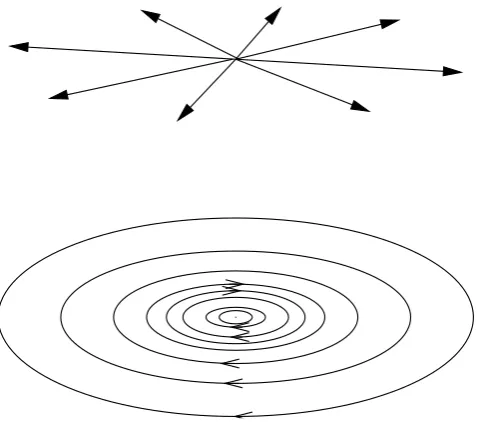
We can represent the ionospheric electric fields and cur-rents by using special non-local vector basis functions, Carte-sian Elementary Current Systems (CECS). CECS were intro-duced by Amm (1997) and although the name “CECS” refers to current systems, they can be used to represent any smooth enough 2-dimensional vector field in planar geometry. There are two different types of CECS, one is divergence-free (DF) and the other curl-free (CF). Together they form a complete set of basis functions. The elementary systems, illustrated in Fig. 1, are defined as
Edf = V
df
2πρ0eˆφp (9)
Ecf = V
cf
2πρ0eˆρp. (10)
Hereρ0=q(x−x
p)2+(y−yp)2 is the distance between the
Fig. 1. Schematic presentation of curl-free (upper) and
divergence-free (lower) Cartesian elementary current systems (CECS).
Vcf andVdf are called the scaling factors of the CF and DF CECS, respectively.
The elementary systems are defined in such a way, that the CF CECS has a Diracδ-function divergence and the DF CECS aδ-function curl at its pole,
∇ ·Ecf =Vcfδ(x−xp) δ(y−yp)
(∇ ×Edf)z=Vdfδ(x−xp) δ(y−yp).
By placing a sufficient number of CF and DF CECS at different locations of the plane, one can construct any 2-dimensional vector field from its sources and curls, in ac-cordance with Helmholtz’s theorem. When CECS are used to represent ionospheric currents, the divergence of the CF CECS at its pole is interpreted as a vertically flowing FAC.
In practical numerical calculations vector components are given at some discrete grid points and the CECS systems are placed at another grid. The elementary systems defined in Eqs. (9) and (10) are singular at the origin, where ρ0→0. This means that some care must be used, so that the vectors components are not evaluated in the immediate vicinity of the CECS poles. In practice we use interleaved grids, so that vector components are evaluated only at the corners of the CECS grid cells. Our notation is such that the 2-dimensional vector fields (in this example the electric field) are indicated using italics,E, as done already in the previous sections. The collection of the x- and y-components of the fieldE at all grid points is written in script style, asE, and can be written out as
E=Ex(r1), Ey(r1), Ex(r2), . . . , Ey(rN)
T
. (11)
HereEx(rn)is the x-component ofE at the grid pointrn,
and so on. In a similar fashion the collection of the CECS scaling factors representing the field E is indicated using fraktur style,V, and is defined as
V= h
Vcf(rp1), Vdf(rp1), Vcf(rp2), . . . , Vdf(rpM) iT
.(12) HereVcf(rpm)is the scaling factor of the curl-free CECS
located at grid pointrpm. There is a linear relation between
the vector components and the CECS scaling factors,
E=M·V. (13)
The matrix M depends only on the geometry of the vector and CECS grids, and can be calculated using Eqs. (9) and (10).
3.2 Algorithm for numerical calculations
With the elementary systems we can formulate the approach of Sect. 2.2 in a somewhat different way. The goal is to find such a curl-free current system Jcf that the sum
J=Jeq+Jcf is consistent with a potential electric field. As
before, we assume that the equivalent currents are the same as the divergence-free part of the total currents, Jeq=Jdf,
which is a good approximation at high geomagnetic latitudes. We begin by calculating the electric fieldE1that is
con-sistent with the equivalent currents. This can be written in form (cf. Eq. 7)
E1=(6PJeq−6Heˆz×Jeq)/62, (14)
where, as before,62=62P+6H2. In general, the electric field E1is not curl-free and it may be very different from the real
electric fieldE. It should also be noted that there may be some regions in the analysis area where 6P≈6H≈0, but
Jeq6=0. The easiest way to deal with these regions is to
simply exclude them from the analysis, as the electric field cannot be determined in such regions.
The next step is to divide the field E1 into curl- and
divergence-free parts. As in Eq. (13), there is a linear relation between the vector components and CECS representation of E1,
E1=M1·V1. (15)
The CECS representation, which also gives the division into curl- and divergence-free parts, is easily obtained by in-verting the equation. In the following, we need only the divergence-free part ofE1. The corresponding scaling
fac-tors of the DF CECS are denoted byVdf1 .
The unknown curl-free part of the ionospheric currents, Jcf=−∇8 in Eq. (6), can be constructed using just CF
CECS, as
Jcf =Ncf ·Icf, (16)
grids. The electric fieldE2that is consistent withJcf can be
calculated as in Eq. (14), just replacingJeqbyJcf. Because
also this inverted Ohm’s law is linear, together with Eq. (16) it results in
E2=K2·Icf, (17)
where we have defined a new matrix K2. Both the electric
fieldE2and the curl-free currentsJcf are unknown, but the
matrix K2relating them depends just on the structure of the
calculation grids and on the conductances, and it can be cal-culated using Eqs. (14), (9) and (10).
We may further construct a matrix relation similar to Eq. (15), that dividesE2into curl- and divergence-free parts
using CECS,
E2=M2·V2. (18)
Also in this case the matrix M2depends only on he geometry
of the calculation grids. Now we can use Eqs. (17) and (18) together, and write a relation between the still unknow curl-free currents and CECS representation of the electric field E2,
V2=inv(M2)·K2·Icf. (19)
In the following calculations we need only the divergence-free part ofE2, which is given by the divergence-free CECS
Vdf2 . This part of the scaling factors may be singled out by picking appropiate rows of the matrix L≡inv(M2)·K2.
Equa-tion (19) can be written out as
V2cf(rp1)
V2df(rp1)
V2cf(rp2)
.. . =
L11L12. . .
L21L22. . .
.. . ... . .. ·
Icf(rp1)
Icf(rp2)
Icf(rp3)
.. . . (20)
We see that in this case the divergence-free scaling factors V2df correspond to the odd rows of the matrix L. By defining a new matrix Ldf consisting of the odd rows, we may write a
matrix relation between the divergence-free part of the CECS representation ofE2and the curl-free current system,
Vdf2 =Ldf ·Icf. (21)
If we assume that the total electric fieldE=E1+E2is
curl-free, then the rotational parts ofE1andE2must cancel each
other, so that
Vdf2 = −Vdf1 . (22)
With this condition we can solve the unknown curl-free part of the ionospheric currents as
Icf = −inv(Ldf)·Vdf1 . (23)
As explained above, the vector Vdf1 is obtained from the equivalent currents using Eqs. (14) and (15) and the matrix
Ldf can be contructed through the steps taken in Eqs. (16–
21). After solving Eq. (23) we know the true ionospheric cur-rent densityJ=Jeq+Jcf, and consequently also the electric
field can be solved using Eq. (7).
In summary, the calculation algorithm based on the ele-mentary systems is following:
– Calculate the electric field E1 that is consistent with
Ohm’s law and the equivalent currents. – DivideE1into curl- and divergence-free parts.
– Construct a relation between the unknown curl-free part of the currentJcf and the electric fieldE2 consistent
with it.
– Solve forJcf using the condition that the total electric
fieldE1+E2is curl-free.
This CECS-based calculation algorithm is slightly different from the method presented in Sect. 2.2. For example, in the CECS method we do not have to calculate the gradients of conductances or the curl of the equivalent currents. However, the basic approach of solving the curl-free currents instead of electric potential is the same. In the CECS algorithm we do not have to provide any explicit boundary conditions. The CECS represent the curl and divergence of the vector fields, so the natural and automatically included boundary condition is to assume that the curl and divergence vanish outside the analysis region.
In this article we concentrate on regional studies, but it should be mentioned that the new calculation method can also be used in global scales. The theory presented in Sect. 2.2 does not depend on the specific geometry that is used, and also the numerical algorithm presented in this sec-tion can be used in spherical geometry. The necessary mod-ification is to simply use Spherical elementary current sys-tems (SECS, introduced by Amm, 1997) instead of CECS.
4 Results for a simple electrojet
0 5 10 15
Pedersen conductance
1/
Ω
0 10 20 30 40
Hall conductance
1/
Ω
−20 −15 −10 −5 0
E0
mV/m
E0x E0y
−800 −600 −400 −200 0
J0
A/km
J0x J0y
−400 −200 0 200 400
−0.1 0 0.1
div(E0)
X (km)
V/km
2
−400 −200 0 200 400
−2 −1 0 1 2
FAC0
X (km)
A/km
2
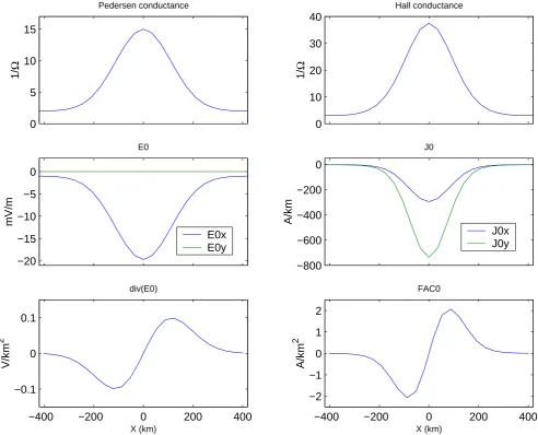
Fig. 2. The electrojet model. Electrojet is uniform in the y-direction. This figure shows the profiles of Pedersen and Hall conductances,
electric fieldE0, ionospheric current densityJ0, divergence of the electric field and FAC in the x-direction.
Calculations are done in a 25×49 grid, with 35 km and 50 km spacing in x- and y-directions, respectively. The KRM equation Eq. (4) is solved using a finite difference scheme with successive overrelaxation (Press et al., 1992, chapter 19). We use a boundary conditionφ=0 for the elec-tric potential in the KRM solution. The new CECS based solution is calculated as outlined in Sect. 3.2. The required matrix inversions are calculated using singular value decom-position (Press et al., 1992, chapter 2).
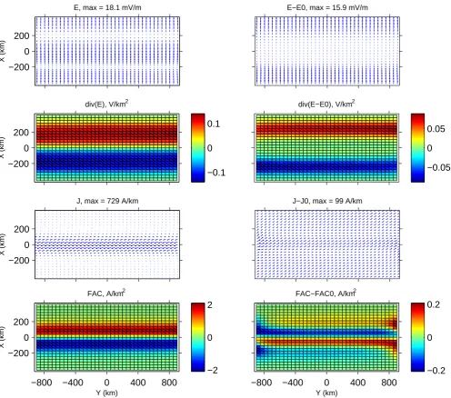
The results of the traditional KRM and the new CECS methods are shown in Figs. 3 and 4, respectively. Both calcu-lation methods produce results that show quite strong bound-ary effects at the eastern and western sides, where the elec-trojet is artificially truncated by the boundaries of the calcu-lation area. For that reason we show the results at a smaller area, omitting 300 km of the calculation grid at both ends of
the electrojet. For both methods four quantities are shown: the calculated electric fieldE, its divergence∇·E, the iono-spheric sheet current densityJ and the FAC. For each vari-able also the difference between the calculated result and the original model is shown.
[image:6.595.52.545.67.465.2]−200 0 200
E, max = 18.1 mV/m
X (km)
E−E0, max = 15.9 mV/m
−0.1 0 0.1
−200 0 200
X (km)
div(E), V/km2
−0.05 0 0.05 div(E−E0), V/km2
−200 0 200
J, max = 729 A/km
X (km)
J−J0, max = 99 A/km
−2 0 2
−800 −400 0 400 800
−200 0 200
Y (km)
X (km)
FAC, A/km2
−0.2 0 0.2
−800 −400 0 400 800
[image:7.595.50.547.61.499.2]Y (km) FAC−FAC0, A/km2
Fig. 3. KRM results for the electrojet model. At each row the KRM result is shown on the left side and the difference between the KRM
result and the original model is on the right side. Rows from top to bottom are: electric field, divergence of the electric field, horizontal currents and FAC. Note the different scales of the vector plots.
but the calculated distribution is much wider than the origi-nal model, leaking outside the actual electrojet. This exam-ple highlights the importance of boundary conditions, when the KRM method is used in local studies. Further examples have been given by Murison et al. (1985). In contrast to the electric field, the horizontal currentJ and vertical FAC are generated very well by the KRM method. This is understand-able, since the currents are concentrated in a narrow strip of enhanced conductivity, where also the electric field was reconstructed accurately. The difference between the KRM result and the original model,J−J0, is an almost uniform
North-East directed current, that has magnitude of∼14% of
the main electrojet. The FAC distribution given by the KRM method is slightly too wide and the peak amplitude is about 10% smaller than in the original model, but on the whole the result is good.
−200 0 200
E, max = 18.9 mV/m
X (km)
E−E0, max = 4.3 mV/m
−0.1 0 0.1
−200 0 200
X (km)
div(E), V/km2
−0.01 0 0.01 div(E−E0), V/km2
−200 0 200
J, max = 765 A/km
X (km)
J−J0, max = 139 A/km
−1 0 1
−800 −400 0 400 800
−200 0 200
Y (km)
X (km)
FAC, A/km2
−0.5 0 0.5
−800 −400 0 400 800
[image:8.595.47.544.60.501.2]Y (km) FAC−FAC0, A/km2
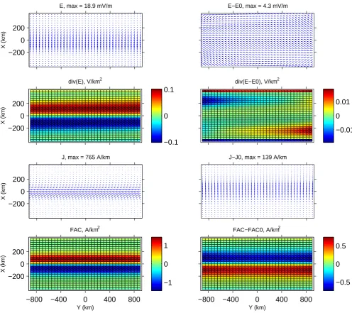
Fig. 4. Results of the CECS method for the electrojet model. Layout is similar to Fig. 3. Note the different scales of the vector plots.
there is also a clear asymmetry in the East-West direction, which results from the sudden termination of the electrojet at these boundaries. However, the current system seems to be reproduced more poorly than with the KRM method. There is about 15% error in the main electrojet current. Main part of the electrojet consists of the Hall currents, which in this case are the same asJeq. The Pedersen currents are curl-free
and are connected to the FAC system. The CECS method underestimates the divergent Pedersen currents, so that the differenceJ−J0 points almost directly northward and the
FAC given by the CECS method are consistently too small. It should be noted that the CECS basis functions used in this paper are intrinsically 2-dimensional and thus, regardless of the specific application, are not optimally suited for
repre-senting 1-dimensional vector fields in a bounded domain. There exists also a 1-dimensional variant of the elementary systems, used by Vanham¨aki et al. (2003) and Juusola et al. (2006), which offer a much more suitable set of basis func-tions for modeling 1-dimensional structures. However, this approach is not pursued further in this study.
From Figs. 3 and 4 it seems that in this simple example the KRM method does produce somewhat better results forJ and FAC, while the new CECS method is able to generateE and∇·Emore accurately. More quantitative estimate for the accuracy of the two methods can be obtained by calculating the mean error in the results, as
error(a)=h|a−a0|i h|a0|i
Table 1. Errors in the electrojet results calculated by the KRM and CECS methods. Error is calculated using Eq. (24) and data presented in Figs. 3 and 4.
E ∇·E J FAC
KRM 108% 74% 29% 7.5%
CECS 42% 9.1% 24% 40%
Here<>denotes average over the calculation area,a is ei-therE,∇·E,J or FAC anda0 is the corresponding model
value.
The error estimates given by Eq. (24) for the electrojet case are given in Table 1. Before discussing these estimates, some important properties of Eq. (24) should be noted. It is easy to see that only the correct solution has 0% error, and a zero solution (e.g.E=0) has 100% error. However, some solu-tions may have errors>100%, but it is questionable whether they are worse than the zero solution. For example a solu-tion that is very close to the correct one, but spatially dis-placed by just few grid cells may have a very large error as calculated from Eq. (24). With these precautions in mind, Table 1 confirms the previous conclusion that in this exam-ple the new CECS method gives more accurate results for the electric field, whereas the current system (especially FAC) is calculated better with the KRM method. The two methods have almost the same percentual errors in the horizontal cur-rentJ, although the plots ofJ−J0in Figs. 3 and 4 are quite
different.
5 Results for realistic data-based models
In this section we use the KRM and CECS methods with two realistic data-based models, namely the-bands and the westward traveling surge (WTS). These models have been published by Amm (1995) and Amm (1996). They are based on observational data obtained at northern Scandinavia by the Scandinavian Magnetometer Array, the EISCAT radar and the EISCAT magnetometer cross, and the STARE radar. In these more complicated models we cannot identifyJeq
with the Hall currents. Instead we calculate the equivalent currents as the divergence-free part of the total ionospheric current density. We divide the total current into divergence-and curl-free parts using the CECS method, as done for the electric field in Sect. 3.2. In order to avoid committing an inverse crime, i.e. using exactly the same numerical process both in preparing the input data and then solving the inverse problem, we use different grid spacings in the separation and in the actual calculations and also add 2% of normally dis-tributed noise to the resulting equivalent (or divergence-free) currents. The original models are given in a regular grids with 50 km resolution in both x- and y-directions. In the
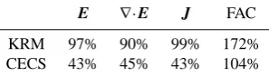
sep-Table 2. Errors in the-band results calculated by the KRM and CECS methods. Error is calculated using Eq. (24) and data pre-sented in Figs. 6 and 7.
E ∇·E J FAC
KRM 97% 90% 99% 172%
CECS 43% 45% 43% 104%
aration of the total model current into divergence- and curl-free parts we use 42 km separation for the CECS, but in the actual calculations the original 50 km separation is used. 5.1 -band
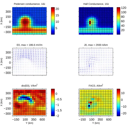
The-band model is illustrated in Fig. 5. The model consists of the Pedersen and Hall conductances, the potential electric fieldE0, the divergence of the electric field and
correspond-ing sheet currentsJ0together with the FAC. Numerical
cal-culations are done in the same way as in Sect. 4.
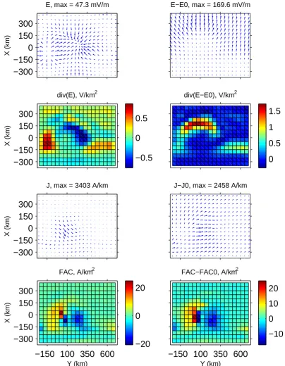
The results obtained using the two methods are given in Figs. 6 and 7. The results are also compared in Table 2, where the error numbers from Eq. (24) are given. In this example the KRM method fails almost completely in generating either the electric field or the horizontal currents, which is again due to the wrong boundary condition. If we want to obtain better results, we must have some additional a priori infor-mation about the structure of the electric field, so that better boundary conditions can be chosen. Although the error num-bers given in Table 2 for∇·Eand FAC are very large, these quantities seem to be produced somewhat better than the vec-tor fields. Especially the divergence of the electric field has reasonable resemblance to the original model, at least qual-itatively. However, the details are not generated correctly, as the area of negative∇·Eat the middle of the calculation grid is too weak and slightly misplaced, and the positive di-vergences at both sides are overestimated. The FAC in the KRM result are mostly concentrated in two small regions, in the same way as in the original model, although neither the exact position nor the magnitude are correct. In the KRM results there are also some weaker and more spread upward and downward FAC areas, that are not present in the original model.
[image:9.595.91.246.111.154.2]5
10
15
20
−300
−150
0
150
300
X (km)
Pedersen conductance, 1/Ω
20
40
60
80
100
120
Hall Conductance, 1/Ω
−300
−150
0
150
300
E0, max = 186.6 mV/m
X (km)
J0, max = 2930 A/km
−2
−1.5
−1
−0.5
0
−150
100
350
600
−300
−150
0
150
300
Y (km)
X (km)
div(E0), V/km2
−20
−10
0
10
−150
100
350
600
[image:10.595.48.555.53.554.2]Y (km) FAC0, A/km2
Fig. 5. The-band model. Pedersen and Hall Conductances, electric fieldE0, ionospheric current densityJ0, divergence of the electric field and FAC. Note the different scales of the vector plots.
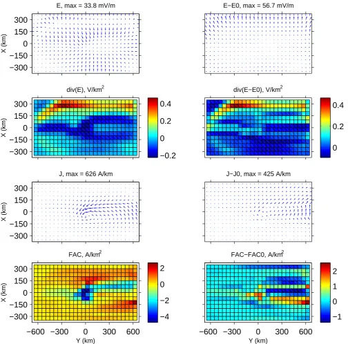
5.2 WTS
The input WTS model is shown in Fig. 8 and the KRM and CECS results are illustrated in Figs. 9 and 10, respectively. The KRM method is able to reproduce the most prominent large scale patterns of∇·E,J and FAC with some accuracy. However, there are also significant deviations from the orig-inal model at some areas and the detailed structure of the WTS system is distorted in the KRM solution. The electric
−300
−150
0
150
300
E, max = 47.3 mV/m
X (km)
E−E0, max = 169.6 mV/m
−0.5
0
0.5
−300
−150
0
150
300
X (km)
div(E), V/km2
0
0.5
1
1.5
div(E−E0), V/km2
−300
−150
0
150
300
J, max = 3403 A/km
X (km)
J−J0, max = 2458 A/km
−20
0
20
−150 100 350 600
−300
−150
0
150
300
Y (km)
X (km)
FAC, A/km2
−10
0
10
20
−150 100 350 600
[image:11.595.93.498.62.583.2]Y (km) FAC−FAC0, A/km2
Fig. 6. KRM results for the-band model. Layout is similar to Fig. 3. Note the different scales of the vector plots.
The solution obtained using the new CECS-based method is shown in Fig. 10. Apart from some deviations at the east-ern boundary and at the North-West corner the CECS method gives very accurate results. It is clear from Figs. 9 and 10 that the CECS method is able to generate all the parameters more accurately than the KRM method. This is confirmed in Ta-ble 3 where the errors calculated using Eq. (24) are given.
−300
−150
0
150
300
E, max = 116.3 mV/m
X (km)
E−E0, max = 81.8 mV/m
−1.5
−1
−0.5
0
−300
−150
0
150
300
X (km)
div(E), V/km2
−0.2
0
0.2
0.4
0.6
0.8
div(E−E0), V/km2
−300
−150
0
150
300
J, max = 2842 A/km
X (km)
J−J0, max = 1032 A/km
−10
0
10
−150 100 350 600
−300
−150
0
150
300
Y (km)
X (km)
FAC, A/km2
−5
0
5
−150 100 350 600
[image:12.595.93.496.57.584.2]Y (km) FAC−FAC0, A/km2
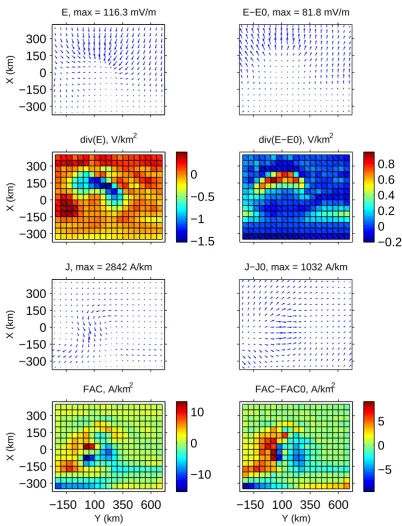
Fig. 7. Results of the CECS method for the-band model. Layout is similar to Fig. 3. Note the different scales of the vector plots.
time derivative of the equivalent currents and then subtract-ing the inductive part fromJeq, as discussed in Sect. 2.2 and
in Vanham¨aki et al. (2007).
6 Summary and conclusions
0
5
10
15
20
−300
−150
0
150
300
X (km)
Pedersen conductance, 1/Ω
20
40
60
80
Hall Conductance, 1/Ω
−300
−150
0
150
300
E0, max = 30.9 mV/m
X (km)
J0, max = 756 A/km
−0.2
−0.1
0
−600
−300
0
300
600
−300
−150
0
150
300
Y (km)
X (km)
div(E0), V/km2
−6
−4
−2
0
2
−600
−300
0
300
600
[image:13.595.48.558.62.480.2]Y (km) FAC0, A/km2
Fig. 8. The WTS model. Layout is similar to Fig. 5. Note the different scales of the vector plots.
et al. (1981). The new method introduced here differs from the KRM method in two important ways. Firstly, the primary unknown to be solved in the new method is the curl-free part of the ionospheric current system, whereas the KRM method formulates the problem in terms of an electric potential. Sec-ondly, in the numerical implementation we use the Carte-sian elementary current systems (CECS), that offer a con-venient way to represent 2-dimensional vector fields, espe-cially when the vector fields have to be divided into curl- and divergence-free parts. These new features lead to a different formulation of the problem, as explained in detail in Sects. 2 and 3.
In this article we concentrated on regional studies, where magnetic measurements and estimates of the ionospheric conductances are available only at a limited region of few hundred or thousand km across. While the KRM method
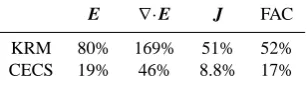
Table 3. Errors in the WTS results calculated by the KRM and CECS methods. Error is calculated using Eq. (24) and data pre-sented in Figs. 9 and 10.
E ∇·E J FAC
KRM 80% 169% 51% 52%
CECS 19% 46% 8.8% 17%
[image:13.595.352.506.574.617.2]−300
−150
0
150
300
E, max = 33.8 mV/m
X (km)
E−E0, max = 56.7 mV/m
−0.2
0
0.2
0.4
−300
−150
0
150
300
X (km)
div(E), V/km2
0
0.2
0.4
div(E−E0), V/km2−300
−150
0
150
300
J, max = 626 A/km
X (km)
J−J0, max = 425 A/km
−4
−2
0
2
−600 −300
0
300
600
−300
−150
0
150
300
Y (km)
X (km)
FAC, A/km2
−1
0
1
2
−600 −300
0
300
600
[image:14.595.48.553.61.559.2]Y (km) FAC−FAC0, A/km2
Fig. 9. KRM results for the WTS model. Layout is similar to Fig. 3. Note the different scales of the vector plots.
(Eq. 8) that makes better use of the information contained in the input equivalent currents than the KRM formulation. An-other advantage is that with CECS the boundary conditions are implemented in a natural way, without having to specify any explicit values for the vector fields or potentials at the boundaries. Thus we expect the new method to be more suit-able for regional studies than the traditional KRM method. The new calculation method may also be used in global stud-ies, as mentioned in Sect. 3.
−300
−150
0
150
300
E, max = 29.9 mV/m
X (km)
E−E0, max = 20.3 mV/m
−0.2
0
0.2
−300
−150
0
150
300
X (km)
div(E), V/km2
0
0.1
0.2
div(E−E0), V/km2−300
−150
0
150
300
J, max = 729 A/km
X (km)
J−J0, max = 83 A/km
−6
−4
−2
0
2
−600 −300
0
300
600
−300
−150
0
150
300
Y (km)
X (km)
FAC, A/km2
0
1
2
−600 −300
0
300
600
[image:15.595.47.552.61.562.2]Y (km) FAC−FAC0, A/km2
Fig. 10. Results of the CECS method for the WTS model. Layout is similar to Fig. 3. Note the different scales of the vector plots.
CECS basis functions are not optimal for representing es-sentially 1-dimensional structures, as discussed in Sect. 4. However, in the three data-based test cases, which show full 2-dimensional variability, the new CECS method was clearly superior to the traditional KRM method. The error estimates calculated using Eq. (24) show that the errors in the CECS results are around 20%–40% in the model cases, whereas the errors in the KRM results are significantly larger. However, it should be mentioned that in these examples we used the
We conclude that the new CECS-based calculation method is well suitable for regional studies and seems to produce more accurate results than the traditional KRM method. One possible topic for a future study is a more thorough compar-ison between the CECS method and the local AMIE-KRM code mentioned in Sect. 2.1. Also a systematic evaluation of the uncertainties caused by inaccurate conductance estimates would be useful when interpreting the results.
Acknowledgements. The authors would like to thank A. Viljanen for his valuable comments on the manuscript. The work of H. Van-ham¨aki was supported by the Finnish Graduate School in Astron-omy and Space Physics.
Topical Editor M. Pinnock thanks H. Wang and A. Aikio for their help in evaluating this paper.
References
Ahn, B.-H., Richmond, A. D., Kamide, Y., et al.: An ionospheric conductance model based on ground magnetic disturbance data, J. Geophys. Res., 103, 14 769–14 780, 1998.
Aksnes, A., Amm, O., Stadsnes, J., et al.: Ionospheric conduc-tances derived from satellite measurements of auroral UV and X-ray emissions, and ground-based data: A comparison, Ann. Geophys., 23, 343–358, 2005,
http://www.ann-geophys.net/23/343/2005/.
Amm O.: Direct determination of the local ionospheric Hall con-ductance distribution from two-dimensional electric and mag-netic field data: Application of the method using models of typi-cal ionospheric electrodynamic situations, J. Geophys. Res., 100, 21 473–21 488, 1995.
Amm, O.: Improved electrodynamic modeling of an omega band and analysis of its current system, J. Geophys. Res., 101, 2677– 2683, 1996.
Amm, O.: Ionospheric elementary current systems in spherical co-ordinates and their application, J. Geomagnetism and Geoelec-tricity, 49, 947–955, 1997.
Amm, O. and Viljanen, A.: Ionospheric disturbance magnetic field continuation from the ground to the ionosphere using spherical elementary current systems, Earth, Planets Space, 51, 431–440, 1999.
Amm, O., Viljanen, A., Pulkkinen, A., Sillanp¨a¨a, I., and Van-ham¨aki, H.: Methods for combined ground-based and space-based analysis of ionospheric current systems, Proc. Fourth Oer-sted International Science Team Conference, Copenhagen, Den-mark, 23–27 September 2002, p. 181–184, 2003.
Chapman, S. and Bartels, J.: Geomagnetism, vol. II, pp. 1049, Ox-ford University Press, New York, 1940.
Fuller-Rowell, T. J. and Evans, D. S.: Height-integrated Pedersen and Hall conductivity patterns inferred from the TIROS-NOAA satellite data, J. Geophys. Res., 92, 7606–7618, 1987.
Haines, G. V.: Spherical cap harmonic analysis, J. Geophys. Res., 90, 2583–2591, 1985.
Janhunen, P.: Reconstruction of electron precipitation characteris-tics from a set of multiwavelength digital all-sky auroral images, J. Geophys. Res., 106, 18 505–18 516, 2001.
Juusola, L., Amm, O., and Viljanen, A.: One-dimensional elemen-tary current systems and their use for determining ionospheric currents from satellite measurements, Earth, Planets Space, 58, 667–678, 2006.
Kamide, Y., Richmond, A. D., and Matsushita, S.: Estimation of ionospheric electric fields, ionospheric currents, and field-aligned currents from ground magnetic records, J. Geophys. Res., 86, 801–813, 1981.
Kamide, Y., Kihn, E. A., Ridley, A. J., Cliver, E. W., and Kadowaki, Y.: Real-time specifications of the geospace environment, Space Sci. Rev., 107, 307–316, 2003.
Lummerzheim, D., Rees, M. H., Craven, J. D., and Frank, L. A.: Ionosheric conductances derived from DE-1 auroral images, J. Atmos. Terr. Phys., 53, 281–289, 1991.
Murison, M., Richmond, A. D., Matsushita, S., and Baumjohann, W.: Estimation of Ionospheric Electric Fields and Currents From a Regional Magnetometer Array, J. Geophys. Res., 90, 3525– 3530, 1985.
Press W. H., Teukolsky, S. A., Vetterling, W. T., and Flannery, B. P.: Numerical Recipes in Fortran 77, 973 pp., Campridge University Press, Cambridge, 2nd ed., 1992.
Pulkkinen, A., Amm, O., Viljanen, A., and BEAR Working Group: Ionospheric equivalent current distributions determined with the method of spherical elementary current systems, J. Geophys. Res., 108(A2), 1053, doi:10.1029/2001JA005085, 2003. Untiedt, J. and Baumjohann, W.: Studies of polar current systems
using the IMS Scandinavian magnetometer array, Space Sci. Rev., 63, 245–390, 1993.
Richmond, A. D. and Kamide, Y.: Mapping electrodynamic fea-tures of the high-latitude ionosphere from localized observations: Technique, J. Geophys. Res., 93, 5741–5759, 1988.
Vanham¨aki H., Amm, O., and Viljanen, A.: One-dimensional up-ward continuation of the ground magnetic field disturbance us-ing spherical elementary current systems, Earth, Planets Space, 2003.
Vanham¨aki H., Amm, O., and Viljanen, A.: Role of inductive elec-tric fields and currents in dynamical ionospheric situations, Ann. Geophys., 25, 437–455, 2007,