Random constraint satisfaction problems
and replica symmetry breaking
Jian Ding (University of Chicago),
Allan Sly (University of California–Berkeley),
and Nike Sun (Stanford University)
Constraint satisfaction problem
(
CSP
): given a collection of
variables
subject to
constraints
, find a
satisfying assignment
A large subclass of CSPs is NP-complete or NP-hard —
what about ‘average’ or ‘typical’ case? Leads to
random CSPs
Levin ’86
Boolean satisfiability
:
k
-CNF
p
x
1_
x
2_
x
3q ^ p
x
2_
x
4_
x
5q
Natural model of a
random
k
-CNF: sample uniformly from
space of
n
-variable,
m
-clause
k
-CNF formulas
p2nqmk formulasConstraint satisfaction problem
(
CSP
):
given a collection of
variables
subject to
constraints
, find a
satisfying assignment
A large subclass of CSPs is NP-complete or NP-hard —
what about ‘average’ or ‘typical’ case? Leads to
random CSPs
Levin ’86
Boolean satisfiability
:
k
-CNF
p
x
1_
x
2_
x
3q ^ p
x
2_
x
4_
x
5q
Natural model of a
random
k
-CNF: sample uniformly from
space of
n
-variable,
m
-clause
k
-CNF formulas
p2nqmk formulasConstraint satisfaction problem
(
CSP
): given a collection of
variables
subject to
constraints
, find a
satisfying assignment
A large subclass of CSPs is NP-complete or NP-hard —
what about ‘average’ or ‘typical’ case? Leads to
random CSPs
Levin ’86
Boolean satisfiability
:
k
-CNF
p
x
1_
x
2_
x
3q ^ p
x
2_
x
4_
x
5q
Natural model of a
random
k
-CNF: sample uniformly from
space of
n
-variable,
m
-clause
k
-CNF formulas
p2nqmk formulasConstraint satisfaction problem
(
CSP
): given a collection of
variables
subject to
constraints
, find a
satisfying assignment
A large subclass of CSPs is NP-complete or NP-hard —
what about ‘average’ or ‘typical’ case?
Leads to
random CSPs
Levin ’86
Boolean satisfiability
:
k
-CNF
p
x
1_
x
2_
x
3q ^ p
x
2_
x
4_
x
5q
Natural model of a
random
k
-CNF: sample uniformly from
space of
n
-variable,
m
-clause
k
-CNF formulas
p2nqmk formulasConstraint satisfaction problem
(
CSP
): given a collection of
variables
subject to
constraints
, find a
satisfying assignment
A large subclass of CSPs is NP-complete or NP-hard —
what about ‘average’ or ‘typical’ case? Leads to
random CSPs
Levin ’86
Boolean satisfiability
:
k
-CNF
p
x
1_
x
2_
x
3q ^ p
x
2_
x
4_
x
5q
Natural model of a
random
k
-CNF: sample uniformly from
space of
n
-variable,
m
-clause
k
-CNF formulas
p2nqmk formulasConstraint satisfaction problem
(
CSP
): given a collection of
variables
subject to
constraints
, find a
satisfying assignment
A large subclass of CSPs is NP-complete or NP-hard —
what about ‘average’ or ‘typical’ case? Leads to
random CSPs
Levin ’86
Boolean satisfiability
:
k
-CNF
p
x
1_
x
2_
x
3q ^ p
x
2_
x
4_
x
5q
Natural model of a
random
k
-CNF: sample uniformly from
space of
n
-variable,
m
-clause
k
-CNF formulas
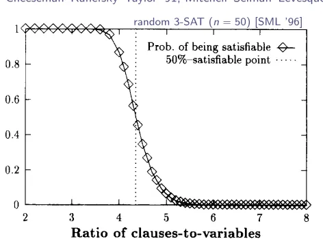
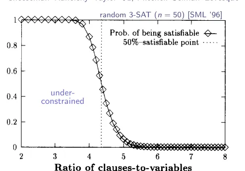
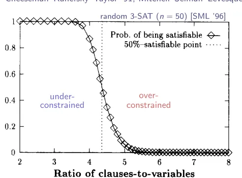
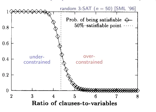
p2nqmk formulasEarly studies noted an empirical
SAT–UNSAT transition
Cheeseman–Kanefsky–Taylor ’91, Mitchell–Selman–Levesque ’92, ’96
random 3-SAT (n“50) [SML ’96]
under-constrained
over-constrained
Early studies noted an empirical
SAT–UNSAT transition
Cheeseman–Kanefsky–Taylor ’91, Mitchell–Selman–Levesque ’92, ’96
random 3-SAT (n“50) [SML ’96]
under-constrained
over-constrained
Early studies noted an empirical
SAT–UNSAT transition
Cheeseman–Kanefsky–Taylor ’91, Mitchell–Selman–Levesque ’92, ’96
22 B. Selman et al./ArrQicial Intelligence 81 (1996) 17-29
Number
bfP calls
2000
0
2 3 4 5 6 7 8
Ratio of clauses-to-variables
Fig. 3. Median DP calls for 50-variable random 3-SAT as a function of the ratio of clauses to variables.
1
0 . 8
0 . 6
Probability
0 . 4
0
2 3 4 5 6 7 8
Ratio of clauses-to-variables
Fig. 4. Probability of satisfiability of 50-variable formulas, as a function of the ratio of clauses to variables.
4). There
is a remarkable
correspondence
between the peak on our curve for number
of recursive calls and the point where the probability
that a formula is satisfiable is
about 0.5. The main empirical conclusion we draw from this is that
the hardest
area for
satisjiability is near the point where 50% of the formulas are satisjiable.
This “50%-satisfiable”
point seems to occur at a fixed ratio of the number of clauses
to the number of variables: when the number of clauses is about 4.3 times the number
of variables. There is a boundary effect for small formulas, and the location gradually
decreases with N: the 50%-point
occurs at
4.55
for formulas with 20 variables; 4.36
for 50 variables;
4.31 for 100 variables and 4.3 for 150 variables
(all empirically
determined).
We conjecture that this ratio approaches about 4.25 for very large numbers
of variables. The peak hardness for DP exhibits the same behavior that we have just
described for the 50-% satisfiable point. These observations
about the 50%-satisfiable
point are confirmed by more detailed experiments
[
10,271.While the performance
of DP can be improved by using clever variable selection
heuristics,
(e.g., [4,38] ), it seems unlikely that such heuristics will
qualitatively
al-
ter the easy-hard-easy
pattern. The formulas in the hard area appear to be the most
challenging for the strategies we
have tested, and we conjecture that they will be for
random 3-SAT (n“50) [SML ’96]
under-constrained
over-constrained
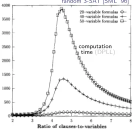
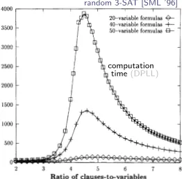
“Hardest” problems seem to occur near SAT–UNSAT transition:
random 3-SAT [SML ’96]
computation time(DPLL)
“Hardest” problems seem to occur near SAT–UNSAT transition:
random 3-SAT [SML ’96]
computation time(DPLL)
“Hardest” problems seem to occur near SAT–UNSAT transition:
B. Sehnun et al. /Art$icial Intelligence 81 (1996) 17-29 21
Number gfIJ
calls
20-variable formulas * 40-variable formulas -I- 50-variable formulas -Sk
2500
2000
1500 1000
500
0
2 3 4 5 6 7 8
Ratio of clauses-to-variables
Fig. 2. Median number of recursive DP calls for random 3-SAT formulas, as a function of the ratio of clauses to variables.
such “outliers” [ 11, it appears to be a more informative statistic for current purposes. 3
In Fig. 2, we see the following pattern: For formulas that are either relatively short or relatively long, DP finishes quickly, but the formulas of medium length take much longer. Since formulas with few clauses are under-consrruined and have many satisfying assignments, an assignment is likely to be found early in the search. Formulas with very many clauses are over-constrained (and usually unsatisfiable), so contradictions are found easily, and a full search can be completed quickly. Finally, formulas in between are much harder because they have relatively few (if any) satisfying assignments, but the empty clause will only be generated after assigning values to many variables, resulting in a deep search tree. Similar under- and over-constrained areas have been found for
random instances of other NP-complete problems [ 8,361.
The curves in Fig. 2 are for all formulas of a given size, that is they are composites of satisfiable and unsatisfiable subsets. In Fig. 3 the median number of calls for 50-variable formulas is factored into satisfiable and unsatisfiable cases, showing that the two sets are quite different. The extremely rare unsatisfiable short formulas are very hard, whereas the rare long satisfiable formulas remain moderately difficult. Thus, the easy parts of the composite distribution appear to be a consequence of a relative abundance of short satisfiable formulas or long unsatisfiable ones.
To understand the hard area in terms of the likelihood of satisfiability, we experimen- tally determined the probability that a random 50-variable instance is satisfiable (Fig.
3 A reasonable question to ask is how big a sample would be required to get a good estimate of the mean.
Because of the potentially exponential nature of the problem, as we increase the samplesize,wemay continue
to find ever larger (but ever rarer) samples that could place the mean anywhere [ 18,331.
random 3-SAT [SML ’96]
computation time(DPLL)
A major advance was the realization that (random) CSPs can be
studied within the framework of
statistical mechanics
M´ezard–Parisi ’85 (weighted matching), ’86 (traveling salesman), Fu–Anderson ’86 (graph partitioning)
The study of CSPs as
models of disordered systems
has
developed into a rich theory, yielding algorithmic advances of
practical significance
survey propagation [M´ezard–Parisi–Zecchina ’02]Theory contains remarkably precise mathematical predictions:
some for
dense
graphs proved in landmark papers
ζp2qlimit of random assignment problem [Aldous ’01]; Parisi formula for SK [Talagrand ’06]; ultrametricity [Panchenko ’13]
while
sparse
graph setting remains less well understood
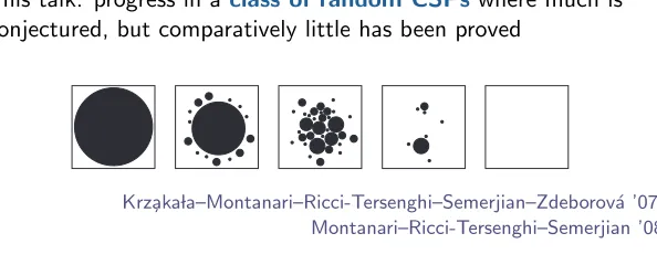
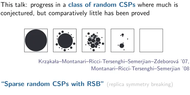
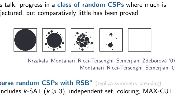
This talk: progress in a
class of random CSPs
where much is
conjectured, but comparatively little has been proved
heuristic implementation of the definition in terms of pure state decomposition (see Eq.4). Generalizing the results of ref. 16, it is possible to show that the two calculations provide identical results. However, the first one is technically simpler and under much better control. As mentioned above we obtain, for allk!4 a value of"d(k) larger than the one quoted in refs. 6 and 11.
Further we determined the distribution of cluster sizeswn, thus
unveiling a third ‘‘condensation’’ phase transition at"c(k)!"d(k) (strict inequality holds fork!4 in SAT andq!4 in coloring, see below). For"!"c(k) the weightswnconcentrate on a logarithmic
scale [namely,"logwnis#(N) with#(N1/2) fluctuations]. Roughly
speaking, the measure is evenly split among an exponential number of clusters.
For"$"c(k) [and!"s(k)] the measure is carried by a subexponential number of clusters. More precisely, the ordered sequence {wn} converges to a well known Poisson-Dirichlet process
{w*n}, first recognized in the spin glass context by Ruelle (26). This
is defined byw*n%xn/&xn, wherexn$0 are the points of a Poisson
process with ratex"1"m(")andm(")!(0, 1). This picture is known in spin glass theory as one-step replica symmetry breaking (1RSB) and has been proven in ref. 27 for some special models. The Parisi 1RSB parameterm(") is monotonically decreasing from 1 to 0 when"increases from"c(k) to"s(k) (see Fig. 3).
Remarkably, the condensation phase transition is also linked to an appropriate notion of correlation decay. Ifi(1), . . . ,i(n)![N] are uniformly random variable indices, then, for"!"c(k) and any fixedn:
!
!
'xi!(
"#)xi)1*. . .xi)n**$#)xi)1**. . .#)xi)n**"30 [5] asN3+. Conversely, the quantity on the left side of Eq.5remains positive for"$"c(k). It is easy to understand that this condition is even weaker than the extremality one (compare Eq.3) in that we probe correlations of finite subsets of the variables. In the next two sections we discuss the calculation of"dand"c.
Dynamic Phase Transition and Gibbs Measure Extremality.A rigorous
calculation of"d(k) along any of the two definitions provided above (compare Eqs.3and4) remains an open problem. Each of the two
approaches has, however, an heuristic implementation that we shall now describe. It can be proved that the two calculations yield equal results as further discussed in the last section.
The approach based on the extremality condition in Eq.3relies on an easy-to-state assumption and typically provides a more precise estimate. We begin by observing that, because of the Markov structure of#!, it is sufficient for Eq.3to hold that the same condition is verified by the correlation betweenxiand the set
of variables at distance exactly!fromi, that we shall keep denoting asx!. The idea is then to consider a large yet finite neighborhood ofi. Given!"!!, the factor graph neighborhood of radius!"around
iconverges in distribution to the radius-!"neighborhood of the root in a well defined random tree factor graphT.
For coloring of random regular graphs, the correct limiting tree modelTis coloring on the infinitel-regular tree. For random
k-SAT,Tis defined by the following construction. Start from the root variable node and connect it tolnew function nodes (clauses),lbeing a Poisson random variable of meank". Connect each of these function nodes withk"1 new variables and repeat. The resulting tree is infinite with nonvanishing probability if"$ 1/k(k"1). Associate a formula to this graph in the usual way, with each variable occurrence being negated independently with probability 1/2.
The basic assumption within the first approach is that the extremality condition in Eq.3can be checked on the correlation between the root and generation-!variables in the tree model. On the tree,#!is defined to be a translation invariant Gibbs measure (17) associated to the infinite factor graphjT(which provides a specification). The correlation between the root and generation-!
variables can be computed through a recursive procedure (defining a sequence of distributionsP"!, see Eq. 15 below). The recursion can be efficiently implemented numerically yielding the values pre-sented in Table 1 fork(resp. q)%4, 5, 6. For largek(resp. q) one can formally expand the equations onP!and obtain:
"d)k*% 2k
k
#
log k,log logk&'d&O$
log logklogk
%&
[6] ld)q*%q-logq&log logq&'d&o)1*. [7] with'd%1 (under a technical assumption of the structure ofP!). The second approach to the determination of"d(k) is based on the ‘‘cavity method’’ (6, 25). It begins by assuming a decomposition in pure states of the form4with two crucial properties: (i) if we denote byWnthe size of thenth cluster (and hencewn%Wn/&Wn),then the number of clusters of sizeWn%eNsgrows approximately
aseN&(s); (ii) for each single-cluster measure#n!, a correlation decay condition of the form3holds.
The approach aims at determining the rate function&(s), com-plexity: the result is expressed in terms of the solution of a distributional fixed point equation. For the sake of simplicity we
jMore precisely#!is obtained as a limit of free boundary measures.
α
d,+α
dα
cα
sFig. 2. Pictorial representation of the different phase transitions in the set of solutions of a rCSP. At"d,,some clusters appear, but for"d,,!"!"dthey comprise
only an exponentially small fraction of solutions. For"d!"!"cthe solutions are split among abouteN&"clusters of sizeeNs". If"c!"!"sthe set of solutions
is dominated by a few large clusters (with strongly fluctuating weights), and above"sthe problem does not admit solutions any more.
Σ(s)
s
αs(k)
αc(k) m(α)
1
0.5
0
Fig. 3. The Parisi 1RSB parameterm(") as a function of the constraint density
". In theInset, the complexity&(s) as a function of the cluster entropy for"% "s(k)"0.1 [the slope at&(s)%0 is"m(")]. Both curves have been computed from the largekexpansion.
10320" www.pnas.org'cgi'doi'10.1073'pnas.0703685104 Krza¸kałaet al. Krz¸aka la–Montanari–Ricci-Tersenghi–Semerjian–Zdeborov´a ’07,
Montanari–Ricci-Tersenghi–Semerjian ’08
“Sparse random CSPs with RSB”
(replica symmetry breaking)This talk: progress in a
class of random CSPs
where much is
conjectured, but comparatively little has been proved
heuristic implementation of the definition in terms of pure state decomposition (see Eq.4). Generalizing the results of ref. 16, it is possible to show that the two calculations provide identical results. However, the first one is technically simpler and under much better control. As mentioned above we obtain, for allk!4 a value of"d(k) larger than the one quoted in refs. 6 and 11.
Further we determined the distribution of cluster sizeswn, thus
unveiling a third ‘‘condensation’’ phase transition at"c(k)!"d(k) (strict inequality holds fork!4 in SAT andq!4 in coloring, see below). For"!"c(k) the weightswnconcentrate on a logarithmic
scale [namely,"logwnis#(N) with#(N1/2) fluctuations]. Roughly
speaking, the measure is evenly split among an exponential number of clusters.
For"$"c(k) [and!"s(k)] the measure is carried by a subexponential number of clusters. More precisely, the ordered sequence {wn} converges to a well known Poisson-Dirichlet process
{w*n}, first recognized in the spin glass context by Ruelle (26). This
is defined byw*n%xn/&xn, wherexn$0 are the points of a Poisson
process with ratex"1"m(")andm(")!(0, 1). This picture is known in spin glass theory as one-step replica symmetry breaking (1RSB) and has been proven in ref. 27 for some special models. The Parisi 1RSB parameterm(") is monotonically decreasing from 1 to 0 when"increases from"c(k) to"s(k) (see Fig. 3).
Remarkably, the condensation phase transition is also linked to an appropriate notion of correlation decay. Ifi(1), . . . ,i(n)![N] are uniformly random variable indices, then, for"!"c(k) and any fixedn:
!
!
'xi!(
"#)xi)1*. . .xi)n**$#)xi)1**. . .#)xi)n**"30 [5] asN3+. Conversely, the quantity on the left side of Eq.5remains positive for"$"c(k). It is easy to understand that this condition is even weaker than the extremality one (compare Eq.3) in that we probe correlations of finite subsets of the variables. In the next two sections we discuss the calculation of"dand"c.
Dynamic Phase Transition and Gibbs Measure Extremality.A rigorous
calculation of"d(k) along any of the two definitions provided above (compare Eqs.3and4) remains an open problem. Each of the two
approaches has, however, an heuristic implementation that we shall now describe. It can be proved that the two calculations yield equal results as further discussed in the last section.
The approach based on the extremality condition in Eq.3relies on an easy-to-state assumption and typically provides a more precise estimate. We begin by observing that, because of the Markov structure of#!, it is sufficient for Eq.3to hold that the same condition is verified by the correlation betweenxiand the set
of variables at distance exactly!fromi, that we shall keep denoting asx!. The idea is then to consider a large yet finite neighborhood ofi. Given!"!!, the factor graph neighborhood of radius!"around
iconverges in distribution to the radius-!"neighborhood of the root in a well defined random tree factor graphT.
For coloring of random regular graphs, the correct limiting tree modelTis coloring on the infinitel-regular tree. For random
k-SAT,Tis defined by the following construction. Start from the root variable node and connect it tolnew function nodes (clauses),lbeing a Poisson random variable of meank". Connect each of these function nodes withk"1 new variables and repeat. The resulting tree is infinite with nonvanishing probability if"$ 1/k(k"1). Associate a formula to this graph in the usual way, with each variable occurrence being negated independently with probability 1/2.
The basic assumption within the first approach is that the extremality condition in Eq.3can be checked on the correlation between the root and generation-!variables in the tree model. On the tree,#!is defined to be a translation invariant Gibbs measure (17) associated to the infinite factor graphjT(which provides a specification). The correlation between the root and generation-!
variables can be computed through a recursive procedure (defining a sequence of distributionsP"!, see Eq. 15 below). The recursion can be efficiently implemented numerically yielding the values pre-sented in Table 1 fork(resp. q)%4, 5, 6. For largek(resp. q) one can formally expand the equations onP!and obtain:
"d)k*% 2k
k
#
log k,log logk&'d&O$
log logklogk
%&
[6] ld)q*%q-logq&log logq&'d&o)1*. [7] with'd%1 (under a technical assumption of the structure ofP!). The second approach to the determination of"d(k) is based on the ‘‘cavity method’’ (6, 25). It begins by assuming a decomposition in pure states of the form4with two crucial properties: (i) if we denote byWnthe size of thenth cluster (and hencewn%Wn/&Wn),then the number of clusters of sizeWn%eNsgrows approximately
aseN&(s); (ii) for each single-cluster measure#n!, a correlation decay condition of the form3holds.
The approach aims at determining the rate function&(s), com-plexity: the result is expressed in terms of the solution of a distributional fixed point equation. For the sake of simplicity we
jMore precisely#!is obtained as a limit of free boundary measures.
α
d,+α
dα
cα
sFig. 2. Pictorial representation of the different phase transitions in the set of solutions of a rCSP. At"d,,some clusters appear, but for"d,,!"!"dthey comprise
only an exponentially small fraction of solutions. For"d!"!"cthe solutions are split among abouteN&"clusters of sizeeNs". If"c!"!"sthe set of solutions
is dominated by a few large clusters (with strongly fluctuating weights), and above"sthe problem does not admit solutions any more.
Σ(s)
s
αs(k)
αc(k) m(α)
1
0.5
0
Fig. 3. The Parisi 1RSB parameterm(") as a function of the constraint density
". In theInset, the complexity&(s) as a function of the cluster entropy for"% "s(k)"0.1 [the slope at&(s)%0 is"m(")]. Both curves have been computed from the largekexpansion.
10320" www.pnas.org'cgi'doi'10.1073'pnas.0703685104 Krza¸kałaet al. Krz¸aka la–Montanari–Ricci-Tersenghi–Semerjian–Zdeborov´a ’07,
Montanari–Ricci-Tersenghi–Semerjian ’08
“Sparse random CSPs with RSB”
(replica symmetry breaking)Prior rigorous work for sparse CSPs
without RSB
: the exact
SAT–UNSAT transition has been determined for several problems:
‚
2-SAT transition
Goerdt ’92, ’96, Chv´atal–Reed ’92, de la Vega ’92 scaling window: Bollob´as–Borgs–Chayes–Kim–Wilson ’01‚
1-in-
k
-SAT transition
Achlioptas–Chtcherba–Istrate–Moore ’01‚
k
-XOR-SAT transition
Dubois–Mandler ’02, Dietzfelbinger–Goerdt– –Mitzenmacher–Montanari–Pagh–Rink ’10, Pittel–Sorkin ’12Prior rigorous work for sparse CSPs
without RSB
:
the exact
SAT–UNSAT transition has been determined for several problems:
‚
2-SAT transition
Goerdt ’92, ’96, Chv´atal–Reed ’92, de la Vega ’92 scaling window: Bollob´as–Borgs–Chayes–Kim–Wilson ’01‚
1-in-
k
-SAT transition
Achlioptas–Chtcherba–Istrate–Moore ’01‚
k
-XOR-SAT transition
Dubois–Mandler ’02, Dietzfelbinger–Goerdt– –Mitzenmacher–Montanari–Pagh–Rink ’10, Pittel–Sorkin ’12Prior rigorous work for sparse CSPs
without RSB
: the exact
SAT–UNSAT transition has been determined for several problems:
‚
2-SAT transition
Goerdt ’92, ’96, Chv´atal–Reed ’92, de la Vega ’92 scaling window: Bollob´as–Borgs–Chayes–Kim–Wilson ’01‚
1-in-
k
-SAT transition
Achlioptas–Chtcherba–Istrate–Moore ’01‚
k
-XOR-SAT transition
Dubois–Mandler ’02, Dietzfelbinger–Goerdt– –Mitzenmacher–Montanari–Pagh–Rink ’10, Pittel–Sorkin ’12Prior rigorous work for sparse CSPs
without RSB
: the exact
SAT–UNSAT transition has been determined for several problems:
‚
2-SAT transition
Goerdt ’92, ’96, Chv´atal–Reed ’92, de la Vega ’92 scaling window: Bollob´as–Borgs–Chayes–Kim–Wilson ’01‚
1-in-
k
-SAT transition
Achlioptas–Chtcherba–Istrate–Moore ’01‚
k
-XOR-SAT transition
Dubois–Mandler ’02, Dietzfelbinger–Goerdt– –Mitzenmacher–Montanari–Pagh–Rink ’10, Pittel–Sorkin ’12For sparse CSPs
with RSB
, threshold behavior long in question
Rigorous bounds on the SAT–UNSAT transition include:
‚
random regular graph independent set
Bollob´as ’81, McKay ’87, Frieze– Luczak ’92, Frieze–Suen ’94, Wormald ’95‚
random graph coloring
Bollob´as ’88,Achlioptas–Naor ’04, Coja-Oghlan–Vilenchik ’13
‚
random
k
-NAE-SAT
Achlioptas–Moore ’02, Coja-Oghlan–Zdeborov´a ’12, Coja-Oghlan–Panagiotou ’12‚
random
k
-SAT
Kirousis–Kranakis–Krizanc–Stamatiou ’97, Achlioptas–Peres ’03, Coja-Oghlan–Panagiotou ’13, Coja-Oghlan ’14 (gap remains in all models: threshold existence not implied)Existence of threshold sequence
(possibly non-convergent) Friedgut ’99Existence of sharp threshold
Bayati–Gamarnik–Tetali ’10For sparse CSPs
with RSB
, threshold behavior long in question
Ri