Demographic Researcha free, expedited, online journal of peer-reviewed research and commentary
in the population sciences published by the Max Planck Institute for Demographic Research Konrad-Zuse Str. 1, D-18057 Rostock·GERMANY www.demographic-research.org
DEMOGRAPHIC RESEARCH
VOLUME 24, ARTICLE 11, PAGES 251-256
PUBLISHED 8 FEBRUARY 2011
http://www.demographic-research.org/Volumes/Vol24/11/ DOI: 10.4054/DemRes.2011.24.11
Formal Relationships 12
Life expectancy:
Lower and upper bounds from surviving
fractions and remaining life expectancy
Joel E. Cohen
This article is part of the Special Collection “Formal Relationships”. Guest Editors are Joshua R. Goldstein and James W. Vaupel.
c
°2011 Joel E. Cohen.
Table of Contents
1 Relationship 252
2 Proof of (2) 253
3 Application to life table of the United States in 2004 254
4 Application to the exponential distribution 255
5 Acknowledgments 256
Demographic Research: Volume 24, Article 11
Formal Relationships 12
Life expectancy:
Lower and upper bounds from surviving
fractions and remaining life expectancy
Joel E. Cohen1
Abstract
We give simple upper and lower bounds on life expectancy. In a life-table population, ife(0)is the life expectancy at birth, M is the median length of life, ande(M)is the expected remaining life at age M, then(M +e(M))/2 ≤ e(0) ≤ M +e(M)/2. In general, for any agex, ife(x)is the expected remaining life at agex, and`(x)is the fraction of a cohort surviving to agexat least, then (x+e(x))·`(x) ≤ e(0) ≤ x+
`(x)·e(x). For any two ages0 ≤w≤x≤ω,(x−w+e(x))·`(x)/`(w)≤e(w)≤ x−w+e(x)·`(x)/`(w). These inequalities give bounds one(0)even without detailed knowledge of the course of mortality prior to agex, provided`(x)can be estimated. Such bounds could be useful for estimating life expectancy when the input of eggs or neonates can be estimated but mortality cannot be observed before late juvenile or early adult ages.
1Laboratory of Populations, Rockefeller & Columbia Universities, 1230 York Avenue, Box 20, New York, NY 10065-6399, USA. E-mail: [email protected]
1. Relationship
The life table`(x), constant in time, with continuous agex, is the proportion of a cohort (whether a birth cohort or a synthetic period cohort) that survives to agexor longer. The maximum possible ageωmay be finite or infinite. By definition,`(0) = 1and`(ω) = 0
and`(x)is non-increasing with increasingx, and therefore is nonnegative since`(ω) = 0. Assume`(x)is a continuous function ofx,0≤x≤ω. The complete expectation of life at agex,e(x), is the average number of years remaining to be lived by those who have attained agex.
We show here thate(0), life expectancy at birth, satisfies, for every agex,
(1) (x+e(x))·`(x)≤e(0)≤x+`(x)·e(x).
More generally, for any two ages0≤w≤x≤ω,
(2) (x−w+e(x))· `(x)
`(w) ≤e(w)≤x−w+e(x)·
`(x)
`(w).
Whenw = 0, (2) reduces to (1). All these inequalities reduce to equality whenx = 0
in (1) orx= win (2) and are strict inequalities ifx > 0orx > wand`(x)is strictly decreasing with increasingx. Subtracting the lower bound in (1) from the upper bound in (1) gives the difference(x−w)(1−`(x)/`(w)). Both factors in this expression increase with the difference in agesx−w, so the closer the age differencex−wis to 0, the closer the lower and upper bounds are toe(w). Also, the higher the probability`(x)/`(w)of survival from agewtox, the closer the lower and upper bounds are toe(w).
The inequalities take a particularly simple form whenw= 0andx=M, the median length of life. Then`(M) = 1/2and
(3) M +e(M)
2 ≤e(0)≤M +
e(M) 2 .
Similarly, whenw= 0andx=U, the upper quartile of length of life, then`(U) = 1/4
and
(4) U+e(U)
4 ≤e(0)≤U+
e(U) 4 .
Also, from (2),
(5) U−M +e(U)
2 ≤e(M)≤U−M+
e(U) 2 .
As a consequence of (1),
Demographic Research: Volume 24, Article 11
These inequalities make it possible to estimate bounds fore(0)without detailed knowl-edge of the course of mortality prior to agex, provided that`(x)can be estimated. Such bounds could be useful in estimating life expectancy when the input of eggs or neonates can be estimated but mortality cannot be observed before late juvenile or early adult ages. The lower the mortality before late juvenile or early adult ages, the more closely the bounds will brackete(0).
2. Proof of (2)
A standard formula (Keyfitz 1968:6) for life expectancy at any agew,0≤w≤ω, is
(7) e(w) = 1
`(w)
Z a=ω
a=w
`(a)da.
Therefore, for any agesw< x,
e(w) = 1
`(w)
Z a=x
a=w
`(a)da+ 1
`(w)
Z a=ω
a=x
`(a)da=T1 +T2.
Since`(x)is non-increasing asxincreases,
(8) T1≥ 1
`(w)
Z a=x
a=w
`(x)da= `(x)
`(w)·(x−w).
(9) T2 = 1
`(w)
Z a=ω
a=x
`(a)da= 1
`(w)
`(x)
`(x)
Z a=ω
a=x
`(a)da= `(x)
`(w)e(x).
Hencee(w)≥(x−w+e(x))·`(x)/`(w), which proves the lower bound in (2). To prove the upper bound in (2), observe that
(10) T1 = 1
`(w)
Z a=x
a=w
`(a)da≤ 1 `(w)
Z a=x
a=w
`(w)da=x−w.
Hencee(w)≤x−w+e(x)·`(x)/`(w). Q.E.D.
3. Application to life table of the United States in 2004
Arias (2007) tabulated`x,qx, andexfor exact ages0,1,2, . . . ,99, and a terminal
catch-all group 100 years or older, for the 2004 United States population. Table 1 compares the life expectancy at birthe(0)with the upper and lower bounds obtained from (1) at selected ages, and Figure 1 shows the comparison at every age. The difference between the lower and upper bounds is less than 1.4 years up to age 40 and then increases rapidly with increasing age. At every age up to 40 years, the upper bound minuse(0)is greater than or equal toe(0)minus the lower bound (excepting ages 35 and 38, where the exceptions are probably artifacts of rounding), while at every age from 41 years onward, the upper bound minuse(0)is strictly less than e(0)minus the lower bound. That is, the lower bound approximatese(0)more closely at younger ages (up to 40 years), while the upper bound approximatese(0)more closely at older ages in this example.
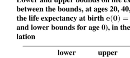
Table 1: Lower and upper bounds on life expectancy at birth and difference between the bounds, at ages 20, 40, 60, and 80 years, compared to the life expectancy at birthe(0) =77.8years (value of the upper and lower bounds for age 0), in the United States’ 2004 total popu-lation
lower upper upper minus age bound bound lower bound
0 77.8 77.8 0.0
20 77.8 78.0 0.3
40 77.1 78.5 1.4
60 72.6 79.8 7.2
80 48.0 84.9 36.9
Demographic Research: Volume 24, Article 11
Figure 1: For the United States total population in 2004, for every agex from 0 to 99 years, upper bounds (rising dark blue dots), lower bounds (falling red solid line), the difference between the upper and the lower bounds (rising cyan dash-dot line), and the life ex-pectancy at birthe(0)(horizontal olive dotted straight line), based on applying (1) to`(x)ande(x)from Arias (2007)
4. Application to the exponential distribution
If the life table is negative exponential with parameterK, i.e.,`(x) = exp(−Kx), then
e(x) = 1/Kfor everyx. The inequalities (1) become
µ x+ 1
K 
e−Kx≤ 1 K ≤x+
e−Kx K .
These inequalities are easily proved without reference to the general case, as follows. Atx= 0, both inequalities are equalities. It is elementary to check that forx > 0the derivative of the lower bound (as a function ofx) is−Kxe−Kx, which is negative, and the
derivative of the upper bound is(1−e−Kx), which is positive, so that strict inequalities
hold for anyx >0.
A referee conjectured that, for the exponential distribution, if x > 0, the error of the lower bound, namely, 1
K −(x+K1)e−Kx, is strictly less than the error of the upper
bound, namely,x+e−Kx
K −K1. By simple algebra, the referee observed, the conjectured
inequality holds if and only iff(x)>0for allx >0, where
f(x) =x−(2/K)(1−exp(−Kx))/(1 + exp(−Kx)).
To prove thatf(x) > 0 when x > 0, we observe thatf(0) = 0 andf(x) = x− ¡2
K ¢
tanh¡Kx
2
¢
. Because dfdx(x) = (tanh¡Kx
2
¢
)2 ≥0and this last inequality is strict if
x > 0, it follows that f(x) > 0 whenx > 0. This proves that the error of the lower bound is less than the error of the upper bound for the exponential distribution when
x >0. Incidentally, sincetanh(x) + tanh(−x) = 0, these same calculations show that
f(x)<0whenx <0.
5. Acknowledgments
I acknowledge with thanks the helpful comments of two referees, the support of U.S. National Science Foundation grants DMS-0443803 and EF-1038337, the assistance of Priscilla K. Rogerson, and the hospitality of the family of William T. Golden during this work.
References
Arias, E. (2007). United States Life Tables, 2004.National Vital Statistics Reports56(9). December 28. Hyattsville, MD: National Center for Health Statistics.