DEMOGRAPHIC RESEARCH
VOLUME 29, ARTICLE 37, PAGES 963-998
PUBLISHED 13 NOVEMBER 2013
http://www.demographic-research.org/Volumes/Vol29/37/ DOI: 10.4054/DemRes.2013.29.37
Research Article
Family policies in the context of low fertility and
social structure
Thomas Fent
Belinda Aparicio Diaz
Alexia Prskawetz
c
2013 Fent, Aparicio Diaz & Prskawetz.
2. The model 966
2.1 Initial population 967
2.2 Budget restrictions and children 967
2.3 Impact of family policies 968
2.4 Endogenous social network 969
2.5 Social effects and intended fertility 970
3. Simulation results 970
4. Summary and conclusions 982
5. Acknowledgements 985
References 986
Appendices 990
A Technical details of the model 990
A1 Initial population 990
A2 Budget restrictions and children 990
A3 Impact of family policies 991
A4 Endogenous social network 991
A5 Social effects and intended fertility 992
B An extended model with two resources 993
C The social multiplier 996
Family policies in the context of low fertility and social structure
Thomas Fent1
Belinda Aparicio Diaz2
Alexia Prskawetz3
Abstract
OBJECTIVE
In this paper we investigate the effectiveness of family policies in the context of the social structure of a population.
METHODS
We use an agent-based model to analyse the impact of policies on individual fertility de-cisions and on fertility at the aggregate level. The crucial features of our model are the interactions between family policies and social structure, the agents’ heterogeneity, and the structure and influence of the social network. This modelling framework allows us to disentangle the direct effect (the alleviation of resource constraints) from the indirect effect (the diffusion of fertility intentions via social ties) of family policies.
RESULTS
Our results indicate that family policies have a positive and significant impact on fertility. In addition, the specific characteristics of the social network and social effects do not only relate to fertility, but also influence the effectiveness of family policies.
CONCLUSIONS
Family policies can only be successful if they are designed to take into account the char-acteristics of the society in which they are implemented.
1Wittgenstein Centre (IIASA, VID/ÖAW, WU), Vienna Institute of Demography/Austrian Academy of
Sciences, Austria. E-mail: [email protected].
2Wittgenstein Centre (IIASA, VID/ÖAW, WU), Vienna Institute of Demography/Austrian Academy of
Sciences, Austria.
3Institute of Mathematical Methods in Economics, Vienna University of Technology, Austria; Wittgenstein
1.
Introduction
Many countries of the Western world have witnessed below-replacement fertility, with fertility rates falling to ever lower levels during the 1980s and 1990s. Despite the slight increases observed in several countries (Myrskylä, Kohler, and Billari 2009; Goldstein, Sobotka, and Jasilioniene 2009), the continuation of current fertility trends may lead to population ageing and shrinkage over the long run. Governments are increasingly in-terested in developing family policies that address the possible causes of these trends. Currently, however, there is no broad consensus on the effectiveness of policies intended to achieve a sustainable increase in — or at least stabilisation of — fertility.
Having assessed data from 22 industrialised countries over the period 1970–1990, Gauthier and Hatzius (1997) found that cash benefits in the form of family allowances are positively related to fertility. McDonald (2006), on the other hand, has argued that prona-talist policies are both expensive and ineffective. After examining Swedish data, Björk-lund (2006) found that the extension of family policies from the mid-1960s to around 1980 raised the level of fertility. Using data from high-income countries in Europe and North America, Feyrer, Sacerdote, and Stern (2008) found that a doubling of spending per child is associated with an increase in fertility of 0.15 children. Gauthier (2007), trying to generalise empirical findings in a comprehensive survey, noted that studies using micro-level data often show that parental and maternity leave schemes have positive effects on completed cohort fertility, while studies using macro-level data typically find that family policies influence the timing of births, rather than the total number of children. However, she inferred that the impact of these schemes tends to be small, and varies depending on the data used and on the type of policies.
and Billari 2006; Balbo and Mills 2011). However, Montgomery and Casterline (1996) claimed that several empirical studies assessing social effects on fertility apply designs that are not capable of accounting for endogenous social network formation.
Our main hypothesis is that social structure, social learning, and social influence mechanisms influence the effectiveness of family policies. Montgomery and Casterline (1996) distinguish between social learning, which means referring to the knowledge and information of others; and social influence, which is based on the desire to avoid con-flict within social groups and the threat of group disintegration. They argue that social networks (i) provide information that expands the set of choices, (ii) demonstrate the con-sequences of behaviour adopted within the group, and (iii) affect individual preferences through social influence effects and conformity pressures. Thus, one individual adopting a certain behaviour may induce a snowball process, with the behaviour spreading from person to person. We build upon this idea, assuming that fertility preferences, and par-ticularly the change in fertility preferences induced by family policies, are also subject to diffusion processes. We integrate the role of social effects into a model of fertility de-cisions and investigate whether and to what extent the effectiveness of family policies is affected by the social structure. More specifically, family policies may have a direct and an indirect effect on fertility. The direct effect is based on the alleviation of resource con-straints, for instance by providing institutional childcare or financial benefits, and allows parents to achieve their intended level of fertility. The indirect effect of family policies rests on the assumption that many people imitate or consult with their friends, siblings, or parents in choosing their intended level of fertility. Local interactions translate into large-scale patterns that again feed back into small groups (Granovetter 1973). Hence, any additional birth resulting from family policies may cause an increase in fertility inten-tions within the peer group of the family giving birth. Policies causing a modest effect on fertility at the individual level may have a large impact at the macro level due to such peer effects (Feyrer, Sacerdote, and Stern 2008). Therefore, we have developed a model that takes social structure into account and investigated the sensitivity of fertility intentions and realisations with respect to family policies and the parameters that distinguish the so-cial structures. With this contribution, we aim to resolve the confusion and disagreement about the effectiveness of family policies by explicitly addressing their twofold impact.
(observed at the macro level) to its full extent. In order to model the impact of family policies on fertility decisions, it is necessary to include the decision mechanism at the micro level, the society at the macro level, the interaction between the micro and macro levels, and the interactions of individuals within their peer groups. Granovetter (1973) stated that the analysis of processes in interpersonal networks provides the most fruitful micro-macro bridge.
Therefore, we apply an agent-based model (ABM) to evaluate the impact of alterna-tive family policies on fertility in the context of social and institutional structures which differ across countries. ABMs offer the opportunity to capture individual heterogeneity with respect to several characteristics and allow us to test hypotheses regarding fertil-ity behaviour in the context of different cultures and different types of family policies. ABMs add a behavioural dimension to the analysis (Morand et al. 2010). While the fo-cus is on the aggregate level (completed fertility), our model is based on the micro level and explains how aggregate-level properties emerge from the behaviour of the agents at the micro level. As the recent literature argues that social interaction is a key factor in shaping fertility decisions and preferences, we explicitly account for peer group effects in our model. Recently, ABMs have been applied in demography to explain mate choice and marriage behaviour (Simão and Todd 2003; Todd and Billari 2003; Todd, Billari, and Simão 2005; Aparicio Diaz and Fent 2006; Billari et al. 2007; Walker and Davis 2013), fertility (Aparicio Diaz et al. 2011), and migration patterns. Baroni, Žamac, and Öberg (2009b); Baroni et al. (2009a) applied ABMs to investigate the role of family policies in Sweden.
The paper is organised as follows. In section 2. we present the model structure, in sec-tion 3. we illustrate the results of the numerical simulasec-tions, in secsec-tion 4. we summarise our findings and offer some conclusions, in Appendix A we discuss technical details, empirical data, and the parameter space, in Appendix B we sketch an extension of our model, in Appendix C we comment on the social muliplier introduced by Becker and Murphy (2000), and in Appendix D we discuss the animation linked to this paper.
2.
The model
with respect to age, household budget, parity, and intended fertility; the social network which links the agents to a small subset of the population and the social effects acting via that network.4 The agents are endowed with a certain amount of time and money which they allocate to satisfy their own and their childrens’ needs. To keep the model simple, we assume that each household considers one unit of time equivalent toγi,t monetary units. This could mean, for example, that working for one unit of time results inγi,tunits of monetary income, or spendingγi,tmonetary units for a babysitter or for domestic aid results in a gain of one time unit. Consequently, we consider only one combined resource stockwi,tfor each household, which is the sum of household income plus the monetary equivalent of non-working time. The explicit modelling of the social network and social effects allows us to capture the direct and the indirect effects of family policies. Our aim is to gain general insights into the impact of family policies on fertility under dif-ferent assumptions regarding the social structure of a population. While we present the main mechanisms of the model in this section, we discuss technical details, sources of empirical data, and the parameter space in Appendix A.
2.1 Initial population
At timeteach agentiis characterised by her agexi,t, household budgetwi,tcapturing the sum of the monetary equivalent of the time budget and the monetary income, paritypi,t, the number of her dependent children (who do not yet have their own income)ni,t, and her intended fertilityfi,t. Agents are assigned a valuezi, which determines the quantile in the age specific income distribution they belong to. We assume that the agents remain in the same quantile over their entire lives while still progessing to higher income levels as they age.
2.2 Budget restrictions and children
The agent’s own consumption (of time and money),ci,t, is assumed to be a concave func-tion of the household budget,ci,t=σ
√
wi,t, and the consumption level ofni,tdependent
children is defined asc(i,tni,t) = ni,tτ
√
wi,t. Thus, consumption levels of children and parents rise more slowly than linearly with household budget. This is based on empir-ical evidence showing that wealthier households have a higher saving rate (i.e. lower consumption rate) compared to less wealthy households (see e.g. Cutler and Katz 1992;
4We are aware that other characteristics, such as education, also have an impact on childbearing behaviour.
Börsch-Supan and Essig 2005; Fessler, Mooslechner, and Schürz 2012). Comparing two model households with the same number of children but different levels of household budget shows that expenditures per child are higher in the wealthier household which corresponds with the quantity quality literature.
Then, the disposable budgetyi,t— the difference between household budgetwi,tand
consumption — becomesyi,t=wi,t−ci,t−c
(ni,t)
i,t . If the household’s intended fertility exceeds the actual parity,
fi,t> pi,t, (1)
and the disposable budget is equal to or greater than the estimated needs of an additional child,
yi,t≥τ
√
wi,t ⇐⇒
√
wi,t≥σ+ (ni,t+ 1)τ, (2)
the agent is exposed to the biological probability (fecundity) of having another child (Leri-don 2004, 2008). In case of a female birth, a new agentkwith agexk,t= 0is generated. This new agent is mutually linked to her mother and her sisters (see 2.4).
Each agent ages by one year in each time step,xi,t+1 =xi,t+ 1, and children will eventually turn into adults who earn their own income. The probability of this transi-tion depends on the agent’s age and is based on age specific labour force participatransi-tion rates. After the child’s transition to adulthood, the number of her mother’s dependent children is reduced by one, but her mother’s parity is unchanged. Moreover, the new adult agent is assigned her own income levelzi, which determines her household budget
wi,t = wi,t(zi, xi,t), her own social network (see 2.4), and her own fertility intentions. Thereafter, she starts to evaluate her fertility intentions according to the inequalities (1) and (2).
2.3 Impact of family policies
Any policy mix,bf+bvw
i,t, greater than zero partially covers the needs ofni,t depen-dent children, c(i,tni,t)=ni,t τ
√
wi,t−bf−bvwi,t, and the disposable budget can be expressed asyi,t =wi,t−σ
√
wi,t−ni,t τ
√
wi,t−bf−bvwi,t
. The necessary condi-tion for having an addicondi-tional child becomes
√
wi,t≥σ+ (ni,t+ 1)
τ− b
f
√ wi,t
−bv√wi,t
. (3)
This inequality embraces the direct effect of family policies, i.e. the alleviation of the budget constraints, which enable parents to realise their fertility intentions.
2.4 Endogenous social network
Individuals communicate about various intimate aspects of their lives if they are closely connected. In the context of our modelling framework, we refer to this group as an agent’s social network or peer group. Fertility intentions and their realisations are discussed among individuals who are connected. This social network is of crucial importance be-cause it connects the micro and the macro levels. Granovetter defined the strength of a tie as a combination of the amount of time, the emotional intensity, the intimacy, and the reciprocal services which characterise the tie. The strength of the tie connecting two in-dividuals is related to the similarity of the connected inin-dividuals. Moreover, the stronger the tie between two individuals, the larger the proportion of individuals to whom they will both be tied (Granovetter 1973).
The mechanisms generating the endogenous social network in this paper are grounded on these theoretical considerations. The similarity of the agents’ characteristics has an impact on the probability of being chosen to join an agent’s social network (Watts, Dodds, and Newman 2002; Aparicio Diaz et al. 2011). We consider age, income, and intended fertility as the characteristics that determine an agent’s social background. Moreover, we assume a certain degree of network transitivity or clustering, i.e. the tendency that two agents who are both connected to the same agent establish a mutual relationship over time (the friends of my friends are also my friends).
2.5 Social effects and intended fertility
Each agent has an intended fertility defined as the sum of current parity and the intended number of additional children. The intended fertility may be altered due to social learning and social influence imposed by the peer group. Like Montgomery and Casterline (1996) we combine social learning and social influence to general social effects. We assume that interpersonal communication about individual fertility preferences, together with the imitation of peers, may shape preferences. Thus, the dynamics of intended fertility are driven by diffusion via local ties. The adaptations of individual fertility intentions capture the indirect effect of family policies. Parents who have additional children because of the direct effect (see 2.3) may subsequently exert social effects on their peers, resulting in an increase in their fertility intentions.
The network influence operates along two dimensions: the degree to which individ-uals express their opinions or perform certain types of behaviour, and the closeness and strength of a relationship. We assume that each link to a peer with a parity higher (lower) than the intended fertility of the focal individualiimplies a chance thatiwill increase (decrease) her own fertility intention. Since we do not explicitly trace the strength of ties connecting individuals, we assume constant probabilities for positive or negative influ-ence. Thus, each tie connecting two individuals may be strong or weak depending on random numbers generated during the simulation.
Our model continues the approaches of Rosero-Bixby and Casterline (1993) and Mont-gomery and Casterline (1996), who applied social learning and social influence mecha-nisms to model the adoption of contraceptive use. Rosero-Bixby and Casterline (1993) used a differential equation model based on the classic, deterministic diffusion model describing the adoption of an innovation. This approach describes the dynamics of the number of adopters at the population level. Such a framework is capable of consider-ing the interactions among peers, but it focuses entirely on population averages and does not allow for individual heterogeneity. Montgomery and Casterline (1996) developed an empirical specification to estimate the impact of socioeconomic determinants, family planning programmes, and peer group behaviour on the individual propensity to adopt contraception. Aparicio Diaz et al. (2011), on the other hand, used an agent-based model to study the impact of peer group interactions on the shift in age specific fertility between 1984 and 2004.
3.
Simulation results
dependent children, intended fertility, and household budget. For all six initial populations the distributions of the individual characteristics are based on the same probabilities but the actual realisations are different. All initial populations consist of 5000 agents. Since we are interested in the role of social structure with regard to the impact of family policies, we vary the level of fixed and proportional family policiesbf andbv, homophilyα, the degree of network transitivitypr2, the weight of intended fertility2, and the strength of
positive and negative social influencepr3andpr4. In particular, we set1= 1,τ = 2.3,
σ = 2.5, κ = 0.7, α = 0.2 : 0.4 : 1.0,5
2 = 0 : 3 : 3, bf = 0 : 0.2 : 2.0,
bv = 0 : 0.04 : 0.28,pr2 = 0.1 : 0.3 : 0.7, andpr3−pr4=−0.06 : 0.02 : 0.06. This
results in 123,552 different sets of parameter combinations. We discuss these parameters and their feasible ranges in Appendix A. We combine each of these parameter combina-tions with each of the six initial populacombina-tions, which means a total of 741,312 simulacombina-tions, and run each simulation for 100 time steps (years). This may be interpreted as applying 88 different sets of family policies (determined by the parametersbf andbv) on 8424 dif-ferent societies (represented byα,2,pr2,pr3,pr3−pr4, and the initial population). For
each simulation run we record completed cohort fertility, intended fertility, and the fertil-ity gap (the difference between intended and completed cohort fertilfertil-ity) on the aggregate level. This section summarises the results obtained from these simulations.
Agent-based simulations allow for experiments that would not be feasible in the real world, and these experiments help us to visualise trends and relationships. The medium range of parameter settings and the medium range of fertility outcomes represent some-what realistic scenarios, while the extreme ends of the parameter range are applied to cap-ture the interdependencies between family policies, network characteristics, and fertility. Because actual fertility depends on the realisation of fertility intentions, we investigate the two components intended fertility and fertility gap independently. The fertility gap indicates to what extent fertility intentions result in actual fertility behaviour. Individuals adapt their fertility intentions if they interact with individuals with higher or lower par-ity. Therefore, the fertility gap allows us to measure the direct effect of family policies, and the comparison of fertility intentions resulting from different policies allows us to measure the indirect effect.
Figure 1 depicts completed cohort fertility, intended fertility, and the fertility gap of those birth cohorts finishing their reproductive period during the last 10 years of the sim-ulation versus fixed (graphs in the left column) and variable (graphs in the right column) family policies.
Figure 1: Completed cohort fertility, intended fertility, and fertility gap by fixed,bf, and variable,bv, family policies.
0 0.5 1 1.5 2
1.2 1.4 1.6 1.8 2 2.2 2.4 2.6
Cohort fertility vs. fixed family policies
bf
all simulations
bv = 0.0
bv = 0.12
bv = 0.28
0 0.05 0.1 0.15 0.2 0.25
1.2 1.4 1.6 1.8 2 2.2 2.4 2.6
Cohort fertility vs. variable family policies
bv
all simulations
bf = 0.0
bf = 1.0
bf = 2.0
0 0.5 1 1.5 2
2 2.2 2.4 2.6 2.8 3
Intended fertility vs. fixed family policies
bf
all simulations
bv = 0.0
bv = 0.12
bv = 0.28
0 0.05 0.1 0.15 0.2 0.25
2 2.2 2.4 2.6 2.8 3
Intended fertility vs. variable family policies
bv
all simulations
bf = 0.0
bf = 1.0
bf = 2.0
0 0.5 1 1.5 2
0 0.1 0.2 0.3 0.4 0.5 0.6 0.7 0.8
Fertility gap vs. fixed family policies
bf
all simulations
bv = 0.0
bv = 0.12
bv = 0.28
0 0.05 0.1 0.15 0.2 0.25
0 0.1 0.2 0.3 0.4 0.5 0.6 0.7 0.8
Fertility gap vs. variable family policies
bv
all simulations
bf = 0.0
bf = 1.0
bf = 2.0
Due to the large number of simulations, the relatively small size of the agent popu-lations (even small countries like e.g. Andorra, Monaco or San Marino have a lot more than 5000 inhabitants), and the long time span of 100 years, there are some outliers devi-ating strongly from the number of simulations. That is why we present averages of many simulation runs in the graphs. Here and in the following figures, the solid line always represents the average over all of the simulations. In the left column, the dashed, dot-ted, and dot-dashed lines show the averages over all simulations with the same level of proportional family policies (bv), and in the right column they depict the averages over all simulations with the same level of fixed family policies (bf). Both the fixed and the variable family policies appear to have a positive influence on cohort fertility, a small positive impact on intended fertility, and a negative impact on the fertility gap. Because the impact of family policies on the fertility gap appears to be more pronounced than the impact on intended fertility, we may conclude that, in our simulation model and for the specific parameter range, the direct effect of family policies is stronger than the indirect effect.
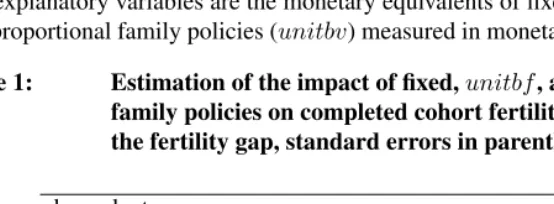
In addition to these graphical visualisations, we present statistical estimates on the impact of family policies in Tables 1 and 2. All of the regression results are based on simulations, and we use ordinary least squares estimation. The dependent variables are completed cohort fertility (ctf r), intended fertility (f), and the fertility gap (gap) of those birth cohorts finishing their reproductive period during the last ten years of the simulation. The explanatory variables are the monetary equivalents of fixed family policies (unitbf) and proportional family policies (unitbv) measured in monetary units per child per year.
Table 1: Estimation of the impact of fixed,unitbf, and variable,unitbv, family policies on completed cohort fertility, intended fertility, and the fertility gap, standard errors in parentheses.
dependent
variable ctf r f gap
.217598*** .0762465*** -.1413515***
unitbf
(.0016135) (.0024278) (.0009583) .0673663*** .0193482*** -.0480182***
unitbv
(.0002631) (.0003959) (.0001562)
AdjustedR2 0.0979 0.0043 0.1311
Number of observations 741312 741312 741312
*** significant at 1 percent
fertility gap. Fixed family policies show a stronger impact. The coefficient forunitbf
explaining cohort fertility,0.217598, can be interpreted as demonstrating that increasing public investments in children by 1000 Euro per child and year would increase cohort fertility by about 0.22. However, this result should be interpreted with caution for two reasons. Firstly, all family policy measures in our model refer to combined resources capturing the sum of cash plus the monetary equivalent of nonmonetary policies from the viewpoint of the household. Secondly, the parameters determing the social structure do not only influence the fertility level but also the impact of family policies. We will show this in Table 2.
Figures 2 and 3 again depict cohort fertility, intended fertility, and the fertility gap versus fixed and proportional family policies. In Figure 2 dashed, dotted, and dot-dashed lines indicate different levels of agents’ homophilyα, in Figure 3 they indicate the differ-ence between the probabilities of being infludiffer-enced by peers with higher or lower parity,
pr3−pr4(see A5).
The graphs reveal that homophilyαhas a visible impact on completed cohort fertility and intended fertility but only a small impact on the fertility gap. Thus, we conclude that the level of homophily in a society has an impact on the indirect effect of family poli-cies, i.e. on the transmission of changes in fertility intentions caused by family policies. The differencepr3−pr4has a positive impact on completed cohort fertility and on the
fertility gap, and a strong positive impact on intended fertility. Thus, the influence mech-anism determined by the parameterspr3andpr4 can alter the indirect effect of family
policies. Figure 4 depicts cohort fertility, intended fertility, and the fertility gap versus the differencepr3−pr4. In the left (right) column, the dashed, dotted, and dot-dashed
lines represent the averages over all simulations with the same level of variable (fixed) family policies. These graphs again illustrate the strong positive impact of the difference
pr3−pr4on the three measures. Moreover, the graphs in the second row show that the
impact ofpr3−pr4on the indirect effect of policies exceeds the impact of the policy mix
(because the range of intended fertility captured by each of the curves is larger than the gap between the curves). The graphs in the third row show that the direct effect of fixed and proportional family policies (depicted by the distances between the lines) and the impact ofpr3−pr4on the fertility gap (illustrated by the range captured by each single
Figure 2: Completed cohort fertility, intended fertility, and the fertility gap by fixed,bf, and variable,bv, family policies and by homophilyα.
0 0.5 1 1.5 2
1.2 1.4 1.6 1.8 2 2.2 2.4 2.6
Cohort fertility vs. fixed family policies
bf
α = 0.2
α = 0.6
α = 1.0
0 0.05 0.1 0.15 0.2 0.25
1.2 1.4 1.6 1.8 2 2.2 2.4 2.6
Cohort fertility vs. variable family policies
bv
α = 0.2
α = 0.6
α = 1.0
0 0.5 1 1.5 2
2 2.2 2.4 2.6 2.8 3
Intended fertility vs. fixed family policies
bf
α = 0.2
α = 0.6
α = 1.0
0 0.05 0.1 0.15 0.2 0.25
2 2.2 2.4 2.6 2.8 3
Intended fertility vs. variable family policies
bv
α = 0.2
α = 0.6
α = 1.0
0 0.5 1 1.5 2
0 0.1 0.2 0.3 0.4 0.5 0.6 0.7 0.8
Fertility gap vs. fixed family policies
bf
α = 0.2
α = 0.6
α = 1.0
0 0.05 0.1 0.15 0.2 0.25
0 0.1 0.2 0.3 0.4 0.5 0.6 0.7 0.8
Fertility gap vs. variable family policies
bv
α = 0.2
α = 0.6
α = 1.0
Figure 3: Completed cohort fertility, intended fertility, and fertility gap by fixed,bf, and variable,bv, family policies andpr3−pr4, the
dif-ference between the probabilities of positive and negative social influence.
0 0.5 1 1.5 2
1.2 1.4 1.6 1.8 2 2.2 2.4 2.6 2.8
Cohort fertility vs. fixed family policies
bf
pr
3 − pr4 = −0.06
pr
3 − pr4 = 0.00
pr3 − pr4 = 0.06
0 0.05 0.1 0.15 0.2 0.25
1.2 1.4 1.6 1.8 2 2.2 2.4 2.6 2.8
Cohort fertility vs. variable family policies
bv
pr3 − pr4 = −0.06
pr
3 − pr4 = 0.00
pr3 − pr4 = 0.06
0 0.5 1 1.5 2
1.8 2 2.2 2.4 2.6 2.8 3 3.2
Intended fertility vs. fixed family policies
bf
pr
3 − pr4 = −0.06
pr
3 − pr4 = 0.00
pr3 − pr4 = 0.06
0 0.05 0.1 0.15 0.2 0.25
1.8 2 2.2 2.4 2.6 2.8 3 3.2
Intended fertility vs. variable family policies
bv
pr3 − pr4 = −0.06
pr
3 − pr4 = 0.00
pr3 − pr4 = 0.06
0 0.5 1 1.5 2
0 0.2 0.4 0.6 0.8 1
Fertility gap vs. fixed family policies
bf
pr
3 − pr4 = −0.06
pr
3 − pr4 = 0.00
pr3 − pr4 = 0.06
0 0.05 0.1 0.15 0.2 0.25
0 0.2 0.4 0.6 0.8 1
Fertility gap vs. variable family policies
bv
pr3 − pr4 = −0.06
pr
3 − pr4 = 0.00
pr3 − pr4 = 0.06
Figure 4: Completed cohort fertility, intended fertility, and fertility gap by pr3−pr4, the difference between the probabilities of positive and
negative social influence and by fixed,bf, and variable,bv, family policies.
−0.06 −0.04 −0.02 0 0.02 0.04 0.06
1.2 1.4 1.6 1.8 2 2.2 2.4 2.6 2.8
Cohort fertility vs. pr3 − pr4
pr3 − pr4
all simulations
bv = 0.0
bv = 0.12
bv = 0.28
−0.06 −0.04 −0.02 0 0.02 0.04 0.06
1.2 1.4 1.6 1.8 2 2.2 2.4 2.6 2.8
Cohort fertility vs. pr3 − pr4
pr3 − pr4
all simulations
bf = 0.0
bf = 1.0
bf = 2.0
−0.06 −0.04 −0.02 0 0.02 0.04 0.06
1.8 2 2.2 2.4 2.6 2.8 3 3.2
Intended fertility vs. pr3 − pr4
pr
3 − pr4
all simulations
bv = 0.0
bv = 0.12
bv = 0.28
−0.06 −0.04 −0.02 0 0.02 0.04 0.06
1.8 2 2.2 2.4 2.6 2.8 3 3.2
Intended fertility vs. pr3 − pr4
pr
3 − pr4
all simulations
bf = 0.0
bf = 1.0
bf = 2.0
−0.060 −0.04 −0.02 0 0.02 0.04 0.06
0.1 0.2 0.3 0.4 0.5 0.6 0.7 0.8
Fertility gap vs. pr
3 − pr4
pr
3 − pr4
all simulations
bv = 0.0
bv = 0.12
bv = 0.28
−0.060 −0.04 −0.02 0 0.02 0.04 0.06
0.1 0.2 0.3 0.4 0.5 0.6 0.7 0.8
Fertility gap vs. pr
3 − pr4
pr
3 − pr4
all simulations
bf = 0.0
bf = 1.0
bf = 2.0
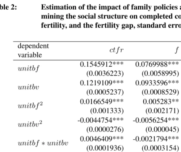
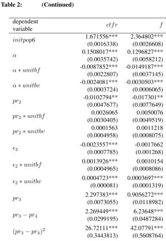
In Table 2, we present statistical estimates on the impact of child support on fer-tility, controlling for network parameters and for social effects. Again, the regression results are based on simulations and we use ordinary least squares estimation. As in the previous regressions, the dependent variables are completed cohort fertility (ctf r), intended fertility (f), and the fertility gap (gap) of those birth cohorts finishing their re-productive period during the last ten years of the simulation. The explanatory variables are unitbf, unitbv, dummy variables initpop2, . . . , initpop6 controlling for the ini-tial pupulation used for each particular simulation run (iniini-tial population 1 serves as the reference group),α,pr2,2,pr3, and pr3−pr4. Moreover, we include the interaction
termsunitbf∗unitbv,α∗unitbf,α∗unitbv,pr2∗unitbf,pr2∗unitbv,2∗unitbf,
2∗unitbv,(pr3−pr4)∗unitbf, and(pr3−pr4)∗unitbv; and the quadratic terms
unitbf2,unitbv2, and(pr
3−pr4)2to control for nonlinear effects.
Table 2: Estimation of the impact of family policies and parameters
deter-mining the social structure on completed cohort fertility, intended fertility, and the fertility gap, standard errors in parentheses
dependent
variable ctf r f gap
0.1545912*** 0.0769988*** -0.0775923***
unitbf
(0.0036223) (0.0058995) (0.0029992) 0.1219109*** 0.0933596*** -0.0285513***
unitbv
(0.0005237) (0.0008529) (0.0004336) 0.0166549*** 0.005283** -0.0113719***
unitbf2
(0.001333) (0.002171) (0.0011037) -0.0044754*** -0.0056254*** -0.0011501***
unitbv2
(0.0000276) (0.000045) (0.0000229) 0.0046409*** -0.0021794*** -0.0068203***
unitbf∗unitbv
(0.0001936) (0.0003154) (0.0001603) 0.5934949*** 0.7079207*** 0.1144258***
initpop2
(0.001634) (0.0026612) (0.0013529) 2.028357*** 3.092795*** 1.064438***
initpop3
(0.001633) (0.0026596) (0.0013521) 1.670658*** 2.363395*** 0.6927377***
initpop4
(0.0016337) (0.0026607) (0.0013527) 1.667212*** 2.359704*** 0.6924919***
initpop5
Table 2: (Continued)
dependent
variable ctf r f gap
1.671556*** 2.364802*** 0.6932458***
initpop6
(0.0016338) (0.0026608) (0.0013527) 0.1508017*** 0.1296827*** -0.021119***
α
(0.0035742) (0.0058212) (0.0029594) -0.0087852*** -0.0149187*** -0.0061335***
α∗unitbf
(0.0022807) (0.0037145) (0.0018884) -0.0024081*** -0.0030503*** -0.0006423**
α∗unitbv
(0.0003724) (0.0006065) (0.0003083) -0.0102794** -0.017301** -0.0070216*
pr2
(0.0047677) (0.0077649) (0.0039476) 0.0026065 0.0050076 0.0024011
pr2∗unitbf
(0.0030405) (0.0049519) (0.0025175) 0.0001563 0.0011218 0.0009655**
pr2∗unitbv
(0.0004958) (0.0008075) (0.0004105)
-0.0023557*** -0.0017662 0.0005895
2
(0.0007785) (0.001268) (0.0006446)
0.0013926*** 0.0010154 -0.0003773
2∗unitbf
(0.0004965) (0.0008086) (0.0004111)
0.0004723*** 0.0003697*** -0.0001026
2∗unitbv
(0.000081) (0.0001319) (0.000067)
2.297383*** 0.9056272*** -1.391756***
pr3
(0.0073055) (0.0118982) (0.006049)
2.269449*** 6.23648*** 3.967031***
pr3−pr4
(0.0299195) (0.0487284) (0.0247732)
26.72111*** 42.07791*** 15.35679*** (pr3−pr4)2
(0.3443813) (0.5608764) (0.2851463)
0.4931002*** 0.1841282*** -0.308972*** (pr3−pr4)∗unitbf
(0.0190671) (0.0310536) (0.0157875)
0.3081202*** 0.2467376*** -0.0613826*** (pr3−pr4)∗unitbv
(0.0031235) (0.0050871) (0.0025862)
-0.3477147*** 0.0317416*** 0.3794563*** constant
(0.0039059) (0.0063614) (0.0032341)
As in the previous estimation,unitbf andunitbvhave a significant positive impact on cohort fertility and intended fertility, and a significant negative impact on the fertility gap. Variable family policies contribute more to the indirect effect (f), while for fixed family policies the direct and indirect effects are nearly equal. The quadratic terms and the interaction of fixed and variable family policies are strongly significant but the coef-ficients are small. The dummy variables representing the initial populations have a big impact and are strongly significant. Thus, the initial conditions at the beginning of the simulation run determine a large portion of the results at the end of the simulation. Ho-mophilyαhas a significant positive impact on cohort fertility and intended fertility, and a significant but small negative impact on the fertility gap. This means homophily op-erates mostly on the indirect effect. The interactions of homophily with family policies
α*unitbfandα*unitbvare strongly significant and the coefficients are all negative and small. Consequently, societies characterised by a high level of homophily tend to higher levels of fertility, the impact of policies on the direct effect (gap) is slightly stronger, and the impact of policies in such societies on the indirect effect (f) is weaker. Network tran-sitivity,pr2, has a negative impact on completed cohort fertility, intended fertility, and
on the fertility gap, and the interactions of transitivity with family policies have a pos-itive impact on all three dependent variables. Like in the case of homophily, this may be interpreted such that societies with a high level of network transitivity tend to lower fertility levels, the impact of policies on the indirect effect (f) is stronger, and the impact of policies on the indirect effect (gap) is weaker. However, in the case of transitivity, not only are the respective coefficients small, but the level of significance is also weak. The weight of intended fertility for calculating the social distance in equation (10),2, has a
small but strongly significant negative impact on cohort fertility, and no significant impact on the other measures. Thus, an increase in2slightly reduces cohort fertility. The
inter-actions with policies, on the other hand, mitigate that effect. The coefficients for cohort fertility have a positive sign and are strongly significant. As expected, the probability of being positively influenced by a peer with higher parity,pr3, has a positive impact on
intended fertility. Moreover, the impact on the fertility gap is significant and negative, resulting in an even stronger positive and significant impact on cohort fertility. The differ-ence between the probabilities of being infludiffer-enced by peers with higher or lower parities, (pr3−pr4), has a strong positive impact on intended fertility and cohort fertility, but
also on the fertility gap. Thus, the increased intentions cannot always be fulfilled due to the budgetary constraints which counteract high fertility intentions. The quadratic term (pr3−pr4)2has an even stronger positive impact on the three dependent variables,
con-firming the convex curves depicted in Figure 4. The interaction(pr3−pr4)∗unitbfhas
the direct and indirect effect of both fixed and variable family policies resulting in higher cohort fertility and a smaller fertility gap. The estimated coefficients show that the indi-rect effect of proportional policies is more sensitive to social effects than is the indiindi-rect effect of fixed policies. This is in agreement with our results regarding the social multi-plier (see C). The direct effect of fixed policies, on the other hand, is more sensitive to social effects than is the direct effect of proportional policies.
The coefficients listed in the second column of Table 2 (completed cohort fertility
ctf r) are based on the empirical specification
ctf r = β0+β1unitbf+β2unitbv+β3unitbf2+β4unitbv2+β5unitbf∗unitbv
+ β6initpop2 +β7initpop3 +β8initpop4 +β9initpop5 +β10initpop6
+ β11α+β12α∗unitbf+β13α∗unitbv
+ β14pr2+β15pr2∗unitbf+β16pr2∗unitbv
+ β172+β182∗unitbf+β192∗unitbv
+ β20pr3+β21(pr3−pr4) +β22(pr3−pr4)2
+ β23(pr3−pr4)∗unitbf+β24(pr3−pr4)∗unitbv. (4)
Then, in a given society characterised by numerical parametersα,pr2,2,pr3, andpr4,
the marginal impact of one monetary unit of fixed family policies (a monetary equivalent of 1000 Euro) on completed cohort fertility can be estimated as the partial derivative of (4) with respect tounitbf,
ctf runitbf = β1+β3unitbf+β5unitbv
+ β12α+β15pr2+β182+β23(pr3−pr4), (5)
and in the same way the marginal impact of one monetary unit of variable family policies on completed cohort fertility may be depicted in the form
ctf runitbv = β2+β4unitbv+β5unitbf
+ β13α+β16pr2+β192+β24(pr3−pr4). (6)
become
ctf runitbf = .1545912 +.0166549∗unitbf+.0046409∗unitbv
−.0087852∗α+.0026065∗pr2+.0013926∗2
+.4931002∗(pr3−pr4) (7)
ctf runitbv = .1219109−.0044754∗unitbv+.0046409∗unitbf
−.0024081∗α+.0001563∗pr2+.0004723∗2
+.3081202∗(pr3−pr4). (8)
Applying the numerical parameters used for the simulations, the mean value of the marginal impactctf runitbf is .195 and the mean value ofctf runitbv is .0978. Hence, providing a monetary equivalent of 1000 Euro per child and year for fixed family policies could raise cohort fertility on average by almost 0.2 and supplying a monetary equiva-lent of 1000 Euro per child and year in terms of proportional family policies could raise cohort fertility on average by nearly 0.1. Depending on the magnitude of the numerical parameters, the pure impact of family policies given by the constant term in (7) and (8) may not only be amplified or damped but even reversed in extreme cases. Comparing the estimated coefficients in Table 1 with the corresponding coefficients in Table 2 re-veals that neglecting the social structure in our simulation model and parameter space results in an overestimation of the impact of fixed policies on completed cohort fertility and on the fertility gap (the coefficients for intended fertility do not differ very much), an underestimation of the impact of proportional policies on completed cohort fertility and on intended fertility, and an overestimation of the impact of proportional policies on the fertility gap.
4.
Summary and conclusions
network, but any agent may indirectly influence any other agent via intermediaries.6 The above-mentioned characteristics, as well as the family policy measures and social effects transmitted via the social network, have an impact on the agents’ fertility intentions and behaviour. The model allows us to carry out experiments to test various combinations of childcare benefits and combine them with different assumptions regarding the underlying social structure.
Our simulations reveal that both fixed and proportional family policies have positive effects on completed cohort fertility and intended fertility and a negative impact on the fertility gap. These findings are in line with empirical studies (Gauthier and Hatzius 1997; Björklund 2006; Gauthier 2007; Feyrer, Sacerdote, and Stern 2008; Egger and Radulescu 2012) and microsimulation models (Kalb and Thoresen 2010). Social networks and social effects are also found to affect fertility, which coincides with empirical results (Bühler and Philipov 2005; Philipov, Spéder, and Billari 2006; Balbo and Mills 2011) and with simulation models (Zamac, Hallberg, and Lindh 2010). Moreover, proportional policies contribute more to the indirect effect (increase in intended fertility) while the contribution of fixed policies to the direct effect (reduction of the gap between intended fertility and completed cohort fertility) and indirect effect are approximately equal. Consequently, the indirect effect of proportional policies is more sensitive to social effects than is the indirect effect of fixed policies. The direct effect of fixed policies, on the other hand, is more sensitive to social effects than is the direct effect of proportional policies. The social multipliers which can be computed for any given level of social effects allows us to quantify to what extent the effectiveness of family policies is mitigated or reinforced by social effects (see C). Our findings that the probability of being positively influenced by a peer with higher parity and the difference between the probabilities of being influenced by peers with higher or lower parities have positive effects on completed cohort fertility and intended fertility, have empirical support from Balbo and Mills (2011), who showed that increased social pressure from parents, relatives, and friends increases the likelihood that a woman will plan to have another child.
Several parameters determining the network and social effects do not only influence fertility itself, but also the effectiveness of family policies, often in a detrimental way. The key element of our model is the combination of family policies and social effects. This allows us to investigate not only the individual effects of policies and social networks but also their interactions. For example, while a higher degree of homophily among the network partners appears to have a positive effect on fertility (intentions and realisations), family policies may be less effective in such a society. Similar results hold for the pa-rameter that characterises the weight put on intended fertility in the selection of the social
6Harary, Norman, and Cartwright (1965) use the term “bridge” for those links that provide the only connection
network, and for the parameters that determine the social influence on intended fertility among network partners. We infer that empirical studies gain from the inclusion of vari-ables depicting the social structure. Kalb and Thoresen (2010), for instance, compare the Australian support scheme which is based on means-tested or income-tested trans-fers and the Nordic scheme of subsidised non-parental care and a universal child benefit schedule. Means-tested transfers and subsidised non-parental care correspond to propor-tional policies in our framework and universal family income support is the equivalent to fixed family policies. Kalb and Thoresen investigate the impact of policiy changes in the context of different labour market characteristics and different behavioural responses in the two countries. They find that reduced childcare fees encourage female labour supply but do not contribute to a more equal distribution of income. They conclude that family policies that redistribute income are more preferable in the Australian context. Parr and Guest (2011) use a longitudinal survey to isolate the effects of family policy changes from general socioeconomic and demographic trends. They conclude that the effect of policy changes is small and not statistically significant.
The main conclusion of our model and simulation exercise is clearly the role of so-cial interaction for the effectiveness of family policies in addition to the direct effect of social interaction on fertility. As well as family policies, social interaction may also in-fluence other determinants of fertility. E.g. the role of economic uncertainty for fertility may be different depending on the social structure of the population. More generally, our modelling framework offers a tool to investigate and disentangle indirect effects of fer-tility determinants from direct ones. In our case the indirect effects work through social interaction and the determinant we are interested in is family policy. However, instead of social interaction or maybe in addition to social interaction other aspects of a society, such as attitudes, norms, and values, may induce an indirect effect on fertility. Similarly the fertility determinant we are interested in, i.e. family policy, may be any other or a set of other family determinants.
A comprehensive review of fertility determinants in advanced societies is given in Balbo, Billari, and Mills (2013). Obviously our model includes only a selection of vari-ables influencing fertility. At the micro/individual level important extensions of our model are the consideration of partners and employment uncertainties. At the meso level not only social interaction but social capital and place of residence may be important charac-teristics to include as well. At the macro level, additional components of family policies (e.g. entitlement to monetary transfers, maternal and paternal leave periods), economic trends, changes in values and attitudes, and the advancement in reproductive technologies are important determinants to be included.
and social pressure on fertility intentions has identified significant cross-country differ-ences (Philipov, Spéder, and Billari 2006; Balbo and Mills 2011), the correct assessment of the effectiveness of family policies requires controlling for social effects. Knack and Keefer (1997) found marked cross country variations in social capital; Wright (1997) noted that the level of homophily varies from country to country; and Kalmijn (1998) inferred that educational homogamy in marriage increased strongly in the United States, but that most countries showed no trend, and that some showed a decrease. Consequently, attempts to transfer a certain policy mix that has proved successful in one country at a certain time to another country or society while ignoring differences in social structure may fail. Family policies can only be successful if they explicitly take into account the characteristics of the society to which they are applied. For instace our simulation shows that in the presence of strong positive social effects fixed policies reduce the fertility gap more effectively, while proportional policies increase intended fertility and vice versa.
We further conclude that cross-country comparisons of different types of family poli-cies should be seen in the context of the social and economic structures. The impact of a certain policy depends on the subset of policies being investigated but comprehen-sive experiments that study any and all possible policy mixes are not feasible in the real world. Moreover, empirical studies addressing the impact of social learning, social pres-sure, and social capital on fertility and fertility intentions show a strong influence of the social structure on intended and actual fertility. We combine the impact of family policies, social networks, and social effects into one unifying framework in order to gain a better understanding of how family policies interact with social and societal structures.
5.
Acknowledgements
References
Aparicio Diaz, B. and Fent, T. (2006). Agent-based computational modelling: Appli-cations in demography, social, economic and environmental sciences. In: Billari, F., Fent, T., Prskawetz, A., and Scheffran, J. (eds.).Contributions to Economics. Springer: 85–116.
Aparicio Diaz, B., Fent, T., Prskawetz, A., and Bernardi, L. (2011). Transition to par-enthood: The role of social interaction and endogenous networks.Demography48(2): 559–579.doi:10.1007/s13524-011-0023-6.
Balbo, N., Billari, F.C., and Mills, M. (2013). Fertility in advanced societies: A review of research. European Journal of Population29(1): 1–38. doi:10.1007/s10680-012-9277-y.
Balbo, N. and Mills, M. (2011). The effects of social capital and social pressure on the intention to have a second or third child in France, Germany, and Bulgaria, 2004-05. Population Studies65(3).
Baroni, E., Eklöf, M., Hallberg, D., Lindh, T., and Žamac, J. (2009a). Fertility deci-sions - Simulation in an agent-based model (IFSIM). In: Zaidi, A., Harding, A., and Williamson, P. (eds.).New Frontiers in Microsimulation Modelling. Ashgate: 265–286.
Baroni, E., Žamac, J., and Öberg, G. (2009b). IFSIM Handbook. Copenhagen: Institute for Futures Studies.
Becker, G.S. and Murphy, K.M. (2000).Social Economics: Market Behavior in a Social Environment. Cambridge, Massachusetts, and London, England: The Belknap Press of Harvard University Press.
Bernardi, L. (2003). Channels of social influence on Reproduction.Population Research and Policy Review22: 527–555.doi:10.1023/B:POPU.0000020892.15221.44.
Billari, F.C., Aparicio Diaz, B., Fent, T., and Prskawetz, A. (2007). The “Wedding-Ring”: An agent-based marriage model based on social interaction. Demographic Research 17(3): 59–82.doi:10.4054/DemRes.2007.17.3.
Björklund, A. (2006). Does family policy affect fertility? Lessons from Sweden.Journal of Population Economics19(1): 3–24.doi:10.1007/s00148-005-0024-0.
Börsch-Supan, A. and Essig, L. (2005). Household saving in Germany: Results of the first SAVE study. In: Wise, D.A. (ed.).Analyses in the Economics of Aging. University of Chicago Press.doi:10.7208/chicago/9780226903217.003.0011.
founda-tions and empirical evidence from Bulgaria. Vienna Yearbook of Population Research 3: 53–81.
Cutler, D.M. and Katz, L.F. (1992). Rising inequality? Changes in the distribution of income and consumption in the 1980s.American Economic Review82(2): 546–551.
Dunbar, R. and Spoors, M. (1995). Social networks, support cliques, and kinship.Human Nature6(3): 273–290.doi:10.1007/BF02734142.
Egger, P.H. and Radulescu, D.M. (2012). Family policy and the number of children: Evidence from a natural experiment.European Journal of Political Economy28: 524– 539. doi:10.1016/j.ejpoleco.2012.05.006.
Fernandez, R. and Fogli, A. (2006). Fertility: The role of culture and family experience. Journal of the European Economic Association 4(2-3): 552–556.
doi:10.1162/jeea.2006.4.2-3.552.
Fessler, P., Mooslechner, P., and Schürz, M. (2012). Household Finance and Consumption Survey des Eurosystems 2010. Erste Ergebnisse für Österreich. Wien: österreichische Nationalbank. (Quartalsheft zur Geld- und Wirtschaftspolitik Q3/12).
Feyrer, J., Sacerdote, B., and Stern, A.D. (2008). Will the stork return to Europe and Japan? Understanding fertility within developed nations. Journal of Economic Per-spectives22(3): 3–22.doi:10.1257/jep.22.3.3.
Gauthier, A.H. (2007). The impact of family policies on fertility in industrialized coun-tries: a review of the literature. Population Research and Policy Review26(3): 323– 346. doi:10.1007/s11113-007-9033-x.
Gauthier, A.H. and Hatzius, J. (1997). Famliy, benefits and fertility: an econometric analysis.Population Studies51(3): 295–306. doi:10.1080/0032472031000150066.
Glaeser, E., Sacerdote, B.I., and Scheinkman, J.A. (2002). The social multiplier. Cam-bridge, Massachusetts: National Bureau of Economic Research. (Working Paper No. 9153).
Goldenberg, J., Libai, B., Moldovan, S., and Muller, E. (2007). The NPV of bad news. International Journal of Research in Marketing 24: 186–200.
doi:10.1016/j.ijresmar.2007.02.003.
Goldstein, J., Sobotka, T., and Jasilioniene, A. (2009). The end of “lowest-low” fer-tility? Population and Development Review 35(4): 663–699. doi:10.1111/j.1728-4457.2009.00304.x.
78(6): 1360–1380.doi:10.1086/225469.
Harary, F., Norman, R., and Cartwright, D. (1965). Structural Models: An Introduction to the Theory of Directed Grap. New York: John Wiley & Sons Inc.
Kalb, G. and Thoresen, T.O. (2010). A comparison of family policy designs of Australia and Norway using microsimulation models. Review of Economics of the Household 8(2): 255–287.doi:10.1007/s11150-009-9076-3.
Kalmijn, M. (1998). Intermarriage and homogamy: Causes, patterns, trends. Annual Review of Sociology24: 395–421.doi:10.1146/annurev.soc.24.1.395.
Knack, S. and Keefer, P. (1997). Does social capital have an economic payoff? Across-country investigation. The Quarterly Journal of Economics 112(4): 1251–1288.
doi:10.1162/003355300555475.
Kohler, H.P., Billari, F., and Ortega, J. (2002). The emergence of lowest-low fertility in Europe during the 1990s. Population and Development Review28(4): 641–680.
doi:10.1111/j.1728-4457.2002.00641.x.
Leridon, H. (2004). Can assisted reproduction technology compensate for the natural decline in fertility with age? A model assessment.Human Reproduction19(7): 1549– 1554.doi:10.1093/humrep/deh304.
Leridon, H. (2008). A new estimate of permanent sterility by age: Steril-ity defined as the inabilSteril-ity to conceive. Population Studies 62(1): 15–24.
doi:10.1080/00324720701804207.
McDonald, P. (2006). Low fertility and the state: The efficacy of policy. Population and Development Review32(3): 485–510. doi:10.1111/j.1728-4457.2006.00134.x.
Montgomery, M.R. and Casterline, J.B. (1996). Social learning, social influence, and new models of fertility. Population and Development Review22(Supplement): 151–175.
doi:10.2307/2808010.
Morand, E., Toulemon, L., Pennec, S., Baggio, R., and Billari, F. (2010). Demographic modelling: The state of the art. Paris: SustainCity. (Working Paper No. 2.1a).
Myrskylä, M., Kohler, H.P., and Billari, F.C. (2009). Advances in development reverse fertility declines.Nature460: 741–743. doi:10.1038/nature08230.
Parr, N. and Guest, R. (2011). The contribution of increases in family benefits to aus-tralia’s early 21st-century fertility increase: An empirical analysis. Demographic Re-search25(6): 215–244. doi:10.4054/DemRes.2011.25.6.
anomie and social capital on fertility intentions in Bulgaria (2002) and Hungary (2001). Population Studies60(3): 289–308.doi:10.1080/00324720600896080.
Rosero-Bixby, L. and Casterline, J.B. (1993). Modelling diffusion effects in fertility transition. Population Studies47(1): 147–167. doi:10.1080/0032472031000146786.
Simão, J. and Todd, P.M. (2003). Emergent patterns of mate choice in human populations. Artificial Life9: 403–417. doi:10.1162/106454603322694843.
Todd, P. and Billari, F.C. (2003). Population-wide marriage patterns produced by indi-vidual mate-search heuristics. In: Billari, F.C. and Fürnkranz, A. (eds.).Agent-based computational demography. Springer: 117–137.
Todd, P., Billari, F.C., and Simão, J. (2005). Aggregate age-at-marriage patterns from individual mate search heuristics.Demography42(3). doi:10.1353/dem.2005.0027.
Walker, L. and Davis, P. (2013). Modelling “marriage markets”: A population-scale im-plementation and parameter test. Journal of Artificial Societies and Social Simulation 16(1).
Watts, D., Dodds, P., and Newman, M. (2002). Idendity and search in social networks. Science296(5571): 1302–1305. doi:10.1126/science.1070120.
Wright, E. (1997). Class Counts: Comparative Studies in Class Analysis. Cambridge: Cambridge University Press.
Zamac, J., Hallberg, D., and Lindh, T. (2010). Low fertility and long-run growth in an economy with a large public sector. European Journal of Population26(2): 183–205.
Appendix
A
Technical details of the model
In this section we elaborate on the technical details, on the empirical data we used to ob-tain the distributions of the agents’ characteristics, and on the feasible parameter space of the model presented in Section 2.. Although we use Austrian data to obtain the distribu-tions of age, parity, income, and intended fertility, the model should not be interpreted as an accurate microsimulation of Austrian society. The intention is to get realistic distribu-tions which resemble typical Western European low-fertility societies.
A1 Initial population
We use census data to obtain an initial age and parity distribution. The parity distribution and the distribution of the age of the children are based on data on the mothers’ age at birth in 2008.7Moreover, we apply data from the income tax statistics8for the distribution of household income. We use age-specific data on the 25% quantile, the median value, and the 75% quantile of the annual net income; and interpolate the data. We then use data from the Gender and Generation Survey (GGS) to estimate the distribution of the desire for additional children given the agents’ age and parity. We define the probabilityπm
i that agentiwants at leastmadditional children(1≤m≤8)and use the logit model
logit(πim) =β0m+β1mxi+βm2 pi (9)
for eachmto estimate the respective probabilities from the GGS data for the initial pop-ulation.
A2 Budget restrictions and children
The numerical parametersσandτneed to be nonnegative and sufficiently small. Negative values would correspond to negative consumption needs, which are unrealistic and would allow for infinite consumption and, in case of negativeτ, for an infinite number of chil-dren. Excessively high values would not allow for any chilchil-dren. For instance,σ=√wi,t (orτ =√wi,t, respectively) means that the agent’s entire budget is needed to cover her own needs (the needs of one child).
In case of a successful live birth, a new agent is generated with a probability depend-ing on the Austrian sex ratio at birth, since our simulation only keeps track of female
individuals. Male children are not implemented as agents within the artificial population, but they contribute to the parity and number of dependent children of their mothers.
Since the distribution of fertility preferences in the artificial society may change over time, we compute for each mthe aggregate share of adult agents with paritypi < m who desire at leastmchildren,Πm
t . We use these shares to update the parametersβ0min
equation (9) every five years according to
βm0,t=β0m
log Πmt
1−Πm t log Πm0
1−Πm
0
,
and the new adult agent’s intended fertility is assigned according to the probabilities
πim= exp(β m
0,t+β1mxi) 1 + exp(βm
0,t+β1mxi)
.
Finally, agents die off with a probability based on the Austrian female life table.
A3 Impact of family policies
From inequalities (1) and (2) it becomes immediately clear that family policies can be effective for those households with unsatisfied fertility preferences and with a funding gap, i.e. households with a disposable budget that is insufficient to meet the needs of an additional child. Thus, it is possible to calculate the level of support needed to in-crease parity by one for each household. However, due to the heterogeneous distribution of (unsatisfied) fertility preferences (which are dynamically adapted via social effects, see 2.5 and A5), the heterogeneous distribution of resources, and the nonlinear relation-ship between resources and needs, it is not possible to calculate the direct impact of family policies at the aggregate level analytically.
The parametersbf andbvneed to be nonnegative. Negative values would mean that the policymaker imposes additional costs or burdens on parents, and the derivation of the neccesary condition for having an additional child (see 2.3) would become invalid. On the other hand, an upper limit for meaningful family policies can be identified at the level at which the family supports per child equal the needs per child,bf+bvw
i,t=τ
√ wi,t.
A4 Endogenous social network
The social distance between agentsiandjis defined as
The parameter1determines the weight of the income difference and2determines the
weight of the differences in the intended fertility of the two agents. Differences in income or intended fertility are ignored when setting the respective parameter zero. To build up the social network, an agent chooses a distancedwith probabilitypr1(d) =cexp(−αd)
and then picks an agent with distancedas a new friend (Watts, Dodds, and Newman 2002; Aparicio Diaz et al. 2011). For this choice, we define another probabilitypr2, which
determines whether this new friend is chosen among those individuals who are not linked to any of the agent’s peers or only among those individuals who are linked to at least one of the agent’s friends. This parameter allows us to adjust the degree of transitivity in the social network which to some degree also serves as a measure of the strength of the ties. The constantcis a normalisation parameter to ensure that the probabilities of all of the feasible distances sum up to one, and the parameterαdetermines the agents’ level of homophily. Ifαis assigned high values, the chances of a connection forming between similar individuals become high. The selecting agent is also added to the network of the selected agent. Thus, we assume a mutual friendship relation which means that the underlying network topology is represented by an undirected graph. This procedure is repeated until the desired number of peers, s, is found. This desired network size is drawn from a log normal distribution (see for instance Dunbar and Spoors 1995, Fig. 1) with means¯= 10and rounded to the nearest integer.
The weights1and2have to be nonnegative but may take any finite number. Very
high values mean a dominance of one characteristic in determining the social distance. The parameterαdetermining the level of homphily may also take any nonnegative value. The probabilitypr2may take any value from the closed interval[0,1].
A5 Social effects and intended fertility
At timetagentihas an intended fertility offi,t, which must be a nonnegative integer, and is defined as the sum of current paritypi,tand the intended additional children. Since we need an approach based at the individual level that allows for nonlinear interaction of positive and negative influence, we implement social effects similar to Goldenberg et al. (2007). We assume that intended fertility increases (decreases) by one with probabil-itypr3 (pr4) due to the social effects exerted by a peer with a parity greater (less) than
the agent’s intended fertility. Then, we computeπi+(π−i ), the number of agentsjwho are linked toiand have a parity greater (less) than the intended fertility of agenti, i.e.
pj,t> fi,t(pj,t< fi,t). Based on these calculations, we compute the probabilities for an agent to be positively or negatively influenced by at least one agent from the peer group,9
9Ifpr
p+i,t= 1−(1−pr3)π
+
i andp−
i,t= 1−(1−pr4)π
−
i . Individuals may be exposed to posi-tive influence, negaposi-tive influence, both posiposi-tive and negaposi-tive influence, or neither. Hence, the probability of being only positively (negatively) influenced becomes(1−p−i,t)p+i,t
(respectively(1−p+i,t)p−i,t) and the probability of being both positively and negatively influenced isp+i,tp−i,t. We use the parameterκ(or (1−κ)) to determine the fraction of individuals who increase (decrease) their intended fertility in the case of mixed influence. Then the probabilities of increasing, decreasing or keeping the intended fertility constant are
pi(fi,t+1=fi,t+ 1) = (1−p−i,t)p
+
i,t+κp
+
i,tp
−
i,t
pi(fi,t+1=fi,t−1) = (1−p+i,t)p
−
i,t+ (1−κ)p
+
i,tp
−
i,t
pi(fi,t+1=fi,t) = (1−p+i,t)(1−p
−
i,t).
The probabilitiespr3andpr4and the parameterκmay take any value from the closed
interval[0,1]. In the case of new products any adopter may influence friends to adopt this product as well (Goldenberg et al. 2007); in our model, actual births are assumed to influence fertility intentions, which do not need to be realised immediately. Thus, we allow for different probabilities for the increase and decrease since the actual parity within the network is usually lower than the desired fertility of the peers. Using the same probability for increasing and decreasing results in a steady bias towards lower levels of intended fertility.
B
An extended model with two resources
In the case of two scarce resources — for example, time and money — the household budget, consumption needs, and family supports provided by the public administration (family policies) must be considered for both components. Let us assume householdi
has a budget ofui,t units of time andvi,t units of money at timet. The agent’s own consumption of time,˜ci,t, and money,cˆi,t, are assumed to be concave functions of the respective household budgets (here and in the following˜denotes quantities of time and ˆrefers to quantities of money),
˜
ci,t= ˜σi,t
√
ui,t and ˆci,t= ˆσi,t
√ vi,t,
and the respective consumption levels ofni,tdependent children are defined as
˜
c(ni,t)=n i,tτ˜i,t
√
ui,t and ˆc(ni,t)=ni,tτˆi,t
√ vi,t.
Therefore, the disposable budgetsy˜i,t andyˆi,t— the difference between the budget and consumption, which can be used, for example, to cover the needs of an additional child — become
˜
yi,t=ui,t−c˜i,t−˜c
(ni,t)
i,t and yˆi,t=vi,t−cˆi,t−ˆc
(ni,t)
i,t .
The necessary conditions to allow for an additional child require that the disposable bud-gets are equal to or greater than the estimated needs of an additional child,y˜i,t≥τ˜i,t
√ ui,t andyˆi,t≥τˆi,t
√
vi,tleading to
√
ui,t≥˜σi,t+ (ni,t+ 1)˜τi,t and
√
vi,t≥σˆi,t+ (ni,t+ 1)ˆτi,t.
The policy maker may provide a mix of fixed family policies per child,˜bfandˆbf, and child benefits proportional to the households resources,˜bvu
i,tandˆbvvi,t. The parameters ˜bf and˜bv determine financial supports, while ˆbf andˆbv represent the additional time
gained by the parents as the result of nonmonetary benefits, such as the provision of public childcare.10 Any policy mix,˜bf+ ˜bvu
i,t,ˆbf+ ˆbvvi,t greater than zero partially covers the demand ofni,tdependent children,
˜ c(ni,t)
i,t = ni,t
˜ τi,t
√
ui,t−˜bf−˜bvui,t
ˆ
c(i,tni,t) = ni,t
ˆ τi,t
√
vi,t−ˆbf−ˆbvvi,t
,
and the disposable budgets can be expressed as
˜
yi,t = ui,t−σ˜
√
ui,t−ni,t
˜ τi,t
√
ui,t−˜bf −˜bvui,t
ˆ
yi,t = vi,t−σˆ
√
vi,t−ni,t
ˆ τi,t
√
vi,t−ˆbf−ˆbvvi,t
.
The necessary conditions for having an additional child become
√
ui,t ≥ σ˜i,t+ (ni,t+ 1) τ˜i,t− ˜bf
√ ui,t
−˜bv√ui,t
!
√
vi,t ≥ σˆi,t+ (ni,t+ 1) τˆi,t− ˆ bf √
vi,t
−ˆbv√vi,t
!
.
10These functional forms suggest that parents with a higher time budget gain more time from nonmonetary
policies. However, the parameterˆbvmay be zero or negative. We include the variable termˆbvv
i,tto avoid