Position-Patch Based Face Hallucination Using Super-Pixel Segmentation and Group Lasso

(1)

POSITION-PATCH BASED FACE HALLUCINATION USING

SUPER-PIXEL SEGMENTATION AND GROUP LASSO

An Undergraduate Research Scholars Thesis by

PENGCHENG PI

Submitted to the Undergraduate Research Scholars program at Texas A&M University

in partial fulfillment of the requirements for the designation as an

UNDERGRADUATE RESEARCH SCHOLAR

Approved by Research Advisor: Dr. Zixiang Xiong

(2)

ABSTRACT

Position-Patch Based Face Hallucination Using Super-Pixel Segmentation and Group Lasso

Pengcheng Pi

Department of Electrical Engineering Texas A&M University

Research Advisor: Dr. Zixiang Xiong Department of Electrical Engineering

Texas A&M University

Traditional super-resolution algorithms utilized samples priors to guide image

reconstruction by image-patch. All of them use square or rectangle patch for acquiring prior information. However, fixed size patches will diminish structural information obtained by

patches. To make patches gain more structural information, we make two adjustments to the face hallucination: superpixel segmentation and Group Lasso. With super-pixel segmentation, we exploit structural features of human faces by segmenting face images into adaptive patches based on their appearances. Group Lasso provides additional structural information through group selection. Our experimental results show that the extra structural information attained by adjustments has a positive impact on the final reconstructed image.

(4)

DEDICATION

(5)

ACKNOWLEDGEMENTS

I would like to thank to my research advisor Professor Zixiang Xiong, Professor Tao Lu. Thanks also go to staff at the undergraduate research scholar program. Finally, thanks to my parents for their constant encouragement and support.

(6)

NOMENCLATURE

HD High Resolution Dictionary

HR High-Resolution

HS High-Resolution Training Human Face Images Set

LD Low Resolution Dictionary

LcR Locality-Constrained Representation LHS Low-Resolution Training Set

LR Low-Resolution

PSNR Peak Signal-To-Noise Ratio

RR Regularizer

RS Region Size

SLIC Simple Linear Iterative Clustering

SR Super Resolution

(7)

CHAPTER I

INTRODUCTION

Super-resolution (Figure. 1) is a method of image enhancement. It generates one or more clear images (high-resolution) from one or more blurred images (low-resolution) based on a prior knowledge.

Figure.1 Super-resolution Example

The main idea (Figure.2) of super-resolution is to provide a more detailed image by increasing the number of pixels per unit area in an image [14]. The core part of this is how to determine values of extended pixels. Practically, one method to achieve this is by

linear-interpolation which includes two parts: training and reconstrution. First, we train a large number of images in high resolution and the same images in corresponding low resolution to setup databases in both high and low resolution (find optimal weight kernel matrix). For reconstructing part, we use the databases to recover a high-resolution image of a vague input.

(8)

Figure.2: Basic Super-resolution Procedure via Interpolation

My work lies in Hallucinating Faces [1], which is one of the topics in super-resolution via linear-interpolation. Our main contribution is to make images of human faces sharper by

collecting partial information of human faces. “Hallucinating Faces” first introduced this topic. During the training part, an important process is to segment each image into small patches so that we can get the training dictionary from these patches locally. Most researches only concentrate on developing new algorithms for recovering images patch by patch with the same segmentation form: a square region of pixels. For example, in the “Position-Patch Based Face Hallucination Via Locality-Constrained Representation” [2], Junjung Jiang et al give us a method to recover patches called locality-constrained representation (LcR), which has better performance than others. Another example of implementing the square segmentation by Cheolkon Jung et al,

(9)

where they use convex optimization to recover patches [3]. A square region segmentation that simply puts a grid on image always omits marginal information of human faces. Specifically, this method decreases structural information captured by patches due to its fixed form. However, superpixel offers us a method to gain more marginal information and structural features by segmenting patches depending on the image’s appearance and spatial components. It is very likely to overcome the blurry margin problems caused by square segmentation.

For reconstruction part, we adopt a new method called group lasso representation. In traditional methods [2-3], every patch in the dictionary has a certain impact on the recovering result for the same position. However, if we divide these items into groups based on their similarity to the target patch, we will provide more structural features and eliminate these patches that have negative effects. Thus, group lasso, which gives different weights on different groups, can achieve this purpose.

(10)

CHAPTER II

METHODS

This part includes reviewing the position patch face hallucination problem, LcR

reconstruction method, SLIC superpixels segmentation, Group Lasso problem, and introducing position-patch based face hallucination using super-pixel segmentation and group lasso.

2.1 Position-Patch Based Face Hallucination

The general frame of position-patch based face hallucination in [2-4] is as follows: Let HDm denoted original images in the training set, m = 1, 2, … , M (the number of samples). For each HDi , we segment it into N square patches as shown in Figure 3. N = IJ, where I and J is the number of patches on each column and row, repectively. On the same position of M training samples, we form a small patches set: { HDm(i, j )|(1 ≤ I ≤ I, 1 ≤ j ≤ J) }. In HD, instead of a p×q matrices, we store each patch as a sorted column vector. For each patch element HDm_{(i, j ),}

we down-sample it by a factor of α and form a low resolution patch set { LDm_{(i, j )|(1 ≤i≤ I,}

1 ≤ j ≤ J) } where each element is a sorted column vector too.

(11)

For each testing low-resolution noised image, we segment it the same way as what we do for low-resolution training images. Let X(i, j) denote the patch on position (i, j) of the testing image and we have:

𝑋(𝑖, 𝑗) = ∑ 𝑤(𝑖, 𝑗) 𝐿𝐷(𝑖, 𝑗) + 𝑒

𝑛𝑢𝑚𝑏𝑒𝑟 𝑜𝑓 𝑠𝑎𝑚𝑝𝑙𝑒𝑠

(1)

where e is error, and w(i, j) is the weight factor for each position, which is approximately the same for high-resolution set and low-resolution set according to [1]. Works in [2-5] offer different methods to solve (1). After getting w(i, j), the reconstruction expression is:

𝑌(𝑖, 𝑗) = ∑ 𝑤(𝑖, 𝑗) 𝐻𝐷(𝑖, 𝑗)

(2)

Y(i, j) is the reconstructed patch for position (i, j). We sort Y(i, j) back to the p×q matrices and map them based on the position (i, j) to construct the final image.

2.2 Superpixels Segmentation

Superpixel offers us a method to gain marginal information of an image by segmenting patches depending on the image’s appearance and spatial components. Currently, there are a lot of algorithms to generate superpixels from images: Quickshift image segmentation [6],

Felzenszwalb’s efficient graph based segmentation [7], Watersheds [8], simple linear iterative clustering (SLIC) [9], and TurboPixels [10].

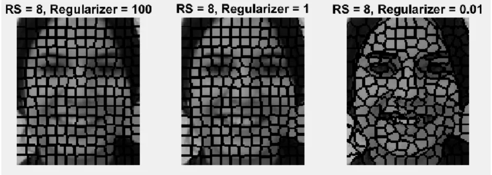
In this research, we choose [9] to generate the patches needed for the training and reconstruction parts for effectiveness. Software package [11] which implements [9], takes two parameters Regularizer (RR) and RegionSize (RS). These two parameters decide the trade-off between clustering and spatial appearance. In Figure 4, we can see how these two parameters affect the segmentation.

(12)

Figure 4: RR and RS effect on the human face images

2.3 Position-Patch Based Face Hallucination Using Super-Pixel Segmentation

Inspired by normal process of traditional position-patch based face hallucination problem such as [2], we first get a uniformed image (UI) of the whole original high-resolution training human face images set (HS):

UI = sum {all images}

number of images (3)

Then we segment the uniformed image via SLIC superpixel segmentation to generate a universal patches’ information set matrices (UM). Figure 5 is the result of segmentation.

Figure 5: segmented uniformed face images

For each original high-resolution image, we first down-sample it and up-sample it back to the high resolution, then combine them as a set of low-resolution training set (LHS). The UM is used as a segmentation template on each HS and LHS to create a HD and a low-resolution

(13)

dictionary (LD). For each input low-resolution image in the testing set, we up-sample it to the high-resolution and apply UM to get its patches. Similar to Section 2.1, for each patch X(i, j), now we have:

𝑋(𝑖, 𝑗) = ∑ 𝑤(𝑖, 𝑗) 𝐿𝐷(𝑖, 𝑗) + 𝑒

(4)

We still suppose w(i, j) remains approximately equal for both high and low resolution images and reconstruct images using (2).

2.4 Algorithm for Position-Patch Based Face Hallucination Using Super-Pixel Segmentation

The detailed algorithm for position-patch based face hallucination using super-pixel segmentation is following:

Input: training image sets HS (sample number is M, each image’s resolution: P×Q), a low-resolution noised image X (resolution: p×q), Regularizer (RR), Region Size (RS).

Output: reconstructed image. 1. Calculate sample factor α

α = √𝑃×𝑄

𝑝×𝑞

2. Calculate uniformed image (UI)

UI = sum {all images} number of images

3. Segment it via SLIC superpixel segmentation (which requires RR and RS) and get UM.

(14)

5. Create two cell HD, LD.

6. For i = 1 to l (number of label in UM) do For i = 1 to M do

 Find all positions in HS i corresponding to label P(i, j) and store pixel values into a column matrices M1.

 Find all positions in LHS i corresponding to label P(i, j) and store pixel values into a column matrices M2.

End For

Add M1 to HD, M2 to LD. End For

7. Up-sample X by 𝛼 and segment using UM 8. For i = 1 to l (number of label in UM) do

 Find all positions corresponding to label X(i, j) and sort it to a column vector X(i) in HSi

 Choose a reconstruction method (e.g., Group Lasso) and calculate w(i, j) for

𝑋(𝑖) = ∑ 𝑤(𝑖) 𝐿𝐷(𝑖) + 𝑒

𝑛𝑢𝑚𝑏𝑒𝑟 𝑜𝑓 𝑠𝑎𝑚𝑝𝑙𝑒𝑠  Reconstruct Y(i, j) via

𝑌(𝑖) = ∑ 𝑤(𝑖) 𝐻𝐷(𝑗)

End For

(15)

2.5 Group Lasso

To solve (1), Jung et al. [3] mentioned a method called sparse representation:

min‖𝑤(𝑖, 𝑗)‖₁ , 𝑠. 𝑡. ‖𝑋(𝑖, 𝑗) − ∑ 𝑤𝑚(𝑖, 𝑗)𝑌𝑚(𝑖, 𝑗) 𝑀 𝑚=1 ‖ 2 2 ≤ 𝜀 (5)

where min‖𝑤(𝑖 ⋅ 𝑗)‖₁ denotes l1-norm. ‖𝑋 − 𝑊𝑌‖22 denotes l2-norm.

[2] proposed following optimization equation which is called locality constrained representation (LcR): min 𝑤 ‖𝑋(𝑖, 𝑗) − ∑ 𝑤𝑚(𝑖, 𝑗)𝑌 𝑚_{(𝑖, 𝑗)} 𝑀 𝑚=1 ‖ 2 2 + 𝜏 ∑ ‖𝑤(𝑖, 𝑗) ∘ 𝑑_𝑚(𝑖, 𝑗)‖22 𝑀 𝑚=1 (6)

Where ∘ denotes a point wise vector product. And d(i, j) is a M-dimensional vector that penalizes the distance between X(i, j) and each training patch at the same position.

𝑑_𝑚(𝑖, 𝑗) = ‖𝑋(𝑖, 𝑗) − 𝑌𝑚_{(𝑖, 𝑗)‖} 2

2 ₍₇₎

[2] offers an algorithm to solve (1).

In this research, we will evaluate a different optimization equation called group lasso:

min 𝑤 ‖𝑋(𝑖, 𝑗) − ∑ 𝑤𝑚(𝑖, 𝑗)𝑌 𝑚_{(𝑖, 𝑗)} 𝑀 𝑚=1 ‖ 2 2 + 𝜆 ∑ 𝑤_𝑖𝑔‖𝑥𝑔‖_𝑞 𝑔𝑠 𝑖=1 (8)

where 𝑤_𝑖𝑔 denotes group weight for that group, 𝑥gdenotes elements in that group, and ‖𝑋‖𝑞 denotes lq-norm (q = 1, 2, …). Software package like [12] can be used to solve this equation.

In LcR optimization equation, (5) gives each element vector different weight based on Euclidean distance to target vector. Those weight will have a certain impact on the final

(16)

eliminate negative impacts of elements vectors who are less likely to target vector by forcing their weights to zero.

There are various standards for choosing elements to different groups. In this research, we tested the standard based on Euclidean distance, Chebyshev distance, Cityblock distance, Cosine distance, and Correlation distance.

The size of group is also a very important property for the final result as well as the value of group weight. We will test some fixed group weight values and a self-adaptive group weight which is defined as:

𝑤_𝑖𝑔 = 1 𝑁∑‖𝑋𝐺𝑖− 𝑋𝑡‖₂ 2 𝑁 𝑖=1 (9)

where N is the group size. For group size, we also adopt a self-adaptive method which sets the group size to be the same as the patch size.

(17)

CHAPTER III

RESULTS

3.1 Database

In my work, human face image samples are chosen from FEI Face Database [14]. The database contains 400 human face images, from which we choose 360 for training and 40 for testing. The original resolution of each image is 120×100. For testing part, we use blurred

samples without noise and smoothed and added noise with variance σ = 5. The images which are used for training and testing have been previously aligned (Figure. 6).

Figure.6: Some training samples

3.2 Impacts of Segmentation Methods

As mentioned in 2.2, there are two parameters regularizer (RR) and regionSize (RS) for SLIC superpixel segmentation. To examine their influence on the final result, we choose low-resolution and noise free test samples. The standard to evaluate reconstruction performance is Peak signal-to-noise ratio (PSNR). The method to solve (1) is LcR. The numerical result is

(18)

RR RS PSNR 0.001 0.01 0.1 1 10 100 6 33.041 33.085 33.101 33.099 33.095 33.095 7 33.061 33.098 33.121 33.126 33.122 33.12 8 33.059 33.112 33.155 33.17 33.171 33.172 9 33.032 33.086 33.111 33.112 33.122 33.1 10 32.961 33.04 33.061 33.047 33.101 33.056 11 32.951 33.042 33.074 33.081 33.054 33.083

Figure.7: Influence of RR and RS on the PSNR of reconstructed images

The original LcR method (with square segmentation) yields a result of 32.95 dB, where we can conclude that our method via superpixel segmentation improves the final reconstructed result. Here are some comparisons between input images and reconstructed images in Figure.8:

Inputs Outputs

(19)

As mentioned in [2], the value of constraint weight 𝜏 plays an important role in the performance of LcR optimization expression. We chose was 𝜏 0.025 which was a reasonable suitable value for the final performance after multiple tests. When we used the original LcR method (square segmentation), we noticed the final performance depended a lot on overlapped patches. If there was no overlapping between patches, PSNR would drop 0.3 dB to 0.5 dB. The patches generated by superpixel segmentation were non-overlapped and still had a good final reconstructed result compared to overlapped patches.

3.3 Group Lasso Performance and Group weights

Using toolbox provided by [12], we can solve (8) by setting relevant parameters. For testing, we chose blurred and noised (σ = 5) low-resolution input images. Instead of traditional face hallucination which used square segmentation method, we chose the algorithm for position-patch based face hallucination using super-pixel segmentation (2.4) to test the relation between Group Lasso’s performance and group weights.

Unlike the test results in 3.2, we found that RR and RS chosen 1000 and 9 yielded better performance under this circumstance (blurred and noise σ = 5 low-resolution inputs). For (8), we chose norm l2(q = 2) for weight constraints. In this experiment, group weights (𝑤_𝑖

𝑔

) were set to multiple fixed value. The test results are shown below (Figure.9):

Group Length = Group Size, λ = 0.03

Group Weight 1000 ₁₅₀₀ ₂₀₀₀ ₂₅₀₀ ₃₀₀₀ ₃₅₀₀ ₄₀₀₀ PSNR(dB) _30.18 _30.21 _30.25 _30.30 _30.21 _30.15 _30.08

(20)

Inputs Outputs

Figure.10: Image Results for Group Weights Test

3.4 Group Lasso Performance and Group Sizes

Group size is another key element in optimization equation (8). We can divide patches of training sets into any number of groups. If the group number equals the number of training samples (each sample is a group for its own), then (8) can be derived as the same form as LcR optimization equation (6). In other words, LcR can be considered as a special case of Group Lasso in l2norm form. For testing, noised (σ = 5), blurred low-resolution images were chosen as

(21)

In this experiment, training patches were divided into two groups, one group size is gs, the other is 360 – gs, where gs were chosen from 1 to 359. Group weight (𝑤_𝑖𝑔) was generated by using self-adaptive formula (9). First and second human face images were chosen as test sample. Test results were shown below (Figure. 11 & Figure. 12):

Max PSNR = 29.48, Max gs = 152 Figure.11: First Image Reconstructed Result

(22)

From Figure.8 and Figure.9, one thing worth noticing is that if the first group (most similar to the target vector) is too small, the reconstructed image’s PSNR would drop

dramatically. Although two image’s best gs are different, the output image’s PSNR is very close to the maximum PSNR in a certain interval of gs where two images’s gs are highly overlapped.

3.5 Group Lasso Performance and Different Choosing Standards

As mentioned in 2.5, the standard for diving elements of the training set into different groups is very important to final reconstructed result. In this experiment, we tested five standards: Euclidean distance, Chebyshev distance, Cityblock distance, Cosine distance, and Correlation distance.

For testing, noise-free and blurred low-resolution images were chosen as inputs. For group lasso expression (8), we chose norm l2(q = 2) for weight constraints. In this experiment,

group weights (𝑤_𝑖𝑔) were generated by the self-adaptive formula (9). Training patches were divided into two groups, one group size is gs, the other is 360 – gs, where gs were chosen from 1 to 359. The results are shown in Figure. 13 – 17.

(23)

Max PSNR = 30.0374, Max gs = 19

Figure.13: First Image Reconstructed Result (Euclidean)

Max PSNR = 29.97, Max gs = 29

(24)

Figure.15: First Image Reconstructed Result (Cityblock)

(25)

Figure.17: First Image Reconstructed Result (Correlation)

From above results, we observed that Euclidean distance as the group choosing standards for patches in the training set can yield best results when we only choose two groups to contain elements. Under this circumstance, the intervals of group size (gs) that generated relative high PSNR are much narrower, which is very different form the results of 3.4.

3.6 Group Lasso Performance and l1, l2, l3 norms

In optimization expression (8), the value for q can be 1, 2… p for the term 𝑤_𝑖𝑔‖𝑥𝑔‖_𝑞 which corresponds to l1-norm, l2-norm, and lp-norm. In this experiment we tested the

performance of l1, l2, l3 norms. For testing, noise-free, blurred low-resolution images were

chosen as inputs. In this experiment, group weights (𝑤_𝑖𝑔) were generated by the self-adaptive formula (9). Training patches were divided into two groups, one group size is gs, the other is 360 – gs, where gs were chosen from 1:359. The results are shown in Figure. 18 – 20.

(26)

Figure.18: First Image Reconstructed Result (l1)

(27)

Figure.20: First Image Reconstructed Result (l3)

(28)

CHAPTER IV

CONCLUSION AND FUTURE WORKS

In this research, we have provided a novel idea to face hallucination this tradition problem: instead of using rigid square segmentation, a more rational segmentation method is applied to generate patches. In addition, we have proven in section 3.2 that such a rational segmentation method can generate better results compared to the original method. To make this segmentation method works more efficiently, we thereby provide an algorithm called position-patch based face hallucination using super-pixel segmentation (section 2.4).

Apart from the influence of choosing different segmentation methods, we also adapt a new optimization constrained expression in the reconstruction part: Group Lasso. Input

parameters of Group Lasso are various. We tested the impacts of group weights, group sizes, as well as the standards of selecting elements in the training patches set for different groups on the final reconstructed result (Section 3.3, 3.4, & 3.5). We find that using adaptive formulas instead of fixed group weight, group size parameters can result in a general better reconstruction image. For the choosing elements standard, we notice that Euclidean distance can generate the highest PSNR value so far.

As we mentioned in section 2.3, we apply a universal superpixel segmentation template to segment all images in the training set. However, this method might still seem to be rigid since each image has its own unique distribution features. Thus, if a more self-adaptive segmentation applied to generate patches, we may improve the final reconstructed result. For example, one reasonable assumption is that the size of each patch generated by such a segmentation method is the same without compromising marginal information extraction. By this means, each image can

(29)

have its own unique segmentation template instead of a universal template for the whole training set.

(30)

REFERENCES

[1] Baker, S., & Kanade, T. (2000). Hallucinating Faces b The pyramid of a lower resolution image. estimating the bottom level of the pyramid. Automatic Face and Gesture

Recognition, 83–88. http://doi.org/10.1109/AFGR.2000.840616

[2] Jiang, J., Hu, R., Han, Z., Lu, T., & Huang, K. (2012). Position-patch based face

hallucination via locality-constrained representation. Proceedings - IEEE International Conference on Multimedia and Expo, 212–217. http://doi.org/10.1109/ICME.2012.152

[3] Jung, C., Jiao, L., Liu, B., & Gong, M. (2011). Position-patch based face hallucination using convex optimization. IEEE Signal Processing Letters, 18(6), 367–370.

http://doi.org/10.1109/LSP.2011.2140370

[4] Ma, X., Zhang, J., & Qi, C. (2010). Hallucinating face by position-patch. Pattern Recognition, 43(6), 2224–2236. https://doi.org/10.1016/j.patcog.2009.12.019

[5] Yang, J., Tang, H., Ma, Y., & Huang, T. (2008). Face hallucination via sparse coding. Proceedings - International Conference on Image Processing, ICIP, (978), 1264–1267. https://doi.org/10.1109/ICIP.2008.4711992

[6] Fulkerson, B., & Soatto, S. (2012). Really quick shift: Image segmentation on a GPU. Lecture Notes in Computer Science (Including Subseries Lecture Notes in Artificial Intelligence and Lecture Notes in Bioinformatics), 6554 LNCS(PART 2), 350–358. http://doi.org/10.1007/978-3-642-35740-4_27

[7] Felzenszwalb, P. F., & Huttenlocher, D. P. (2004). Efficient graph-based image segmentation. International Journal of Computer Vision, 59(2), 167–181. http://doi.org/10.1023/B:VISI.0000022288.19776.77

[8] Machairas, V., Decenciere, E., & Walter, T. (2014). Waterpixels: Superpixels based on the watershed transformation. 2014 IEEE International Conference on Image Processing, ICIP 2014, 4343–4347. http://doi.org/10.1109/ICIP.2014.7025882

[9] Achanta, R., Shaji, A., Smith, K., Lucchi, A., Fua, P., & Süsstrunk, S. (2011). SLIC Superpixels Compared to State-of-the-Art Superpixel Methods. Pattern Analysis and

(31)

Machine Intelligence, IEEE Transactions on, 34(11), 2274–2282. http://doi.org/10.1109/tpami.2012.120

[10] Levinshtein, A. (2009). TurboPixels: Fast Superpixels Using Geometric Flows. IEEE

Transactions on Pattern Analysis and Machine Intelligence, 31, 2290–2297. Retrieved from http://doi.ieeecomputersociety.org/10.1109/TPAMI.2009.96

[11] A. Vedaldi and B. Fulkerson, "VLFeat: An Open and Portable Library of Computer Vision Algorithms," 2008, http://www.vlfeat.org.

[12] J. Liu, S. Ji, and J. Ye. SLEP: Sparse Learning with Efficient Projections. Arizona State University, 2009. http://www.public.asu.edu/~jye02/ Software/SLEP.

[13] C. E. Thomaz and G. A. Giraldi. A new ranking method for Principal Components Analysis and its application to face image analysis, Image and Vision Computing, vol. 28, no. 6, pp. 902-913, June 2010.

[14] K. Nasrollahi and T. B. Moeslund, Super-resolution: A comprehensive survey, vol. 25, no. 6. 2014.

Position-Patch Based Face Hallucination Using Super-Pixel Segmentation and Group Lasso