Solving large systems arising from fractional models by
precondi-tioned methods
Reza Khoshsiar Ghaziani∗
Faculty of Mathematical Sciences, Shahrekord University,
P. O. Box 115, Shahrekord, Iran.
E-mail: [email protected]
Mojtaba Fardi
Faculty of Mathematical Sciences, Shahrekord University,
P. O. Box 115, Shahrekord, Iran.
E-mail: [email protected]
Mehdi Ghasemi
Faculty of Mathematical Sciences, Shahrekord University,
P. O. Box 115, Shahrekord, Iran.
E-mail: [email protected]
Abstract This study develops and analyzes preconditioned Krylov subspace methods for solv-ing discretization of the time-independent space-fractional models. First we apply a shifted Grnwald formulas to obtain a stable finite difference approximation to fractional advection-diffusion equations. Then, we apply two preconditioned iter-ative methods, namely, the preconditioned generalized minimal residual (precon-ditioned GMRES) method and the precon(precon-ditioned conjugate gradient for normal residual(preconditioned CGN) method, to solve the corresponding discritized sys-tems. We make comparisons between the preconditioners commonly used in the parallelization of the preconditioned Krylov subspace methods. The results suggest that preconditioning technique is a promising candidate for solving large-scale linear systems arising from fractional models.
Keywords. Krylov subspace methods, Preconditioning techniques, Fractional model.
2010 Mathematics Subject Classification. 65L05, 34K06, 34K28.
1. Introduction
Recent studies show that fractional advection-diffusion equations provide more ad-equate and accurate description of the movement of solute in an aquifer than the
traditional second-order advectiondiffusion equations do [2,3]. Fractional
advection-diffusion equations are closely related to a continuous time random walk approach, which allows descriptions of particle motions with long-range correlations and is ap-propriate for the description of subsurface solute transport. The most significant
Received: 1 October 2015 ; Accepted: 7 November 2016. ∗Corresponding author.
difference of fractional advection-diffusion equations from their integer analogue is that they generate numerical approximations with full coefficient matrices, which of-ten cause extra numerical difficulties. This is in addition to the common numerical difficulties with their integer analogue. To put the present work in context, we begin by discussing some of the key numerical methods that have been proposed to solve var-ious fractional partial differential equations (FPDEs). In recent years much progress has been made on the development of numerical methods for fractional
advection-diffusion equations. For instance, in [10, 9] a shifted Grnwald formulas was used to
obtain a stable finite difference approximation to fractional advection-diffusion equa-tions. Numerical solution for boundary value problem of fractional order has been
addressed in [12]. A method for solving space-time fractional differential equations is
introduced in [5].
However, the most significant obstacle in the numerical methods for fractional partial differential equations is that these methods generate discrete systems with
full coefficient matrices. ConsequentlyO(N3) account of computations and O(N2)
account of storage are required to solve a problem of sizeN.
Meerschaert and Tadjeran [9], showed that discretisation of the fractional
deriva-tives using standard (non-shifted) Grnwald formulas led to unstable methods when the fractional order. To overcome this, they proposed a method utilising with shifted Grnwald formulas, which they showed to be stable, and first order accurate in space. In more recent times, a number of authors have addressed the issue of high compu-tational expense associated with the solution of FPDEs. Several different approaches have been explored, with many papers employing a mixture of these approaches in various fascinating ways. Krylov subspace methods have been a popular approach, owing to their ability to solve linear systems and compute matrix functions without
the need to operate directly on dense matrices. Yang et al. [21, 22, 23] and Burrage
et al. [4] used Krylov subspace methods for computing matrix functions to solve
frac-tional Laplacian equations. Moroney and Yang [11] and Wang and Wang [20] used
Krylov subspace methods to solve the two-sided space-fractional diffusion equation in one dimension, with the former authors considering nonlinear problems and the latter authors considering linear problems with an advection term.
Preconditioning has been a common theme in many of these papers, since it is well known that Krylov subspace methods generally require an effective preconditioner in
order to perform satisfactorily. Yang et al. [21, 22, 23] developed preconditioners
based on eigenvalue deflation. Burrage et al. [4] considered both algebraic multigrid
and incomplete LU preconditioning. Moroney and Yang [11] developed a banded
preconditioner. A numerical treatment of sparse indefinite systems of linear equations
is given in [13].
In this paper we develop and apply preconditioned methods based on Krylov sub-spaces on linear systems arising from discretized time-independent space-fractional convection-diffusion to obtain the accurate and efficient solution of fractional advection-equations.
methods, namely, GMRES and CGN for solving large-scale linear systems arising from the fractional models. In Section 4 we carry out numerical experiment to investigate the performance of the developed algorithm. Finally, we draw our conclusions in Section 5.
2. The finite difference scheme: Structure of the coefficient matrix
In this section, the implicit finite difference scheme is applied to discretize the time-independent space-fractional convection-diffusion model and the fractional advection-dispersion model, which are obtained from the standard diffusion models by replacing the first order time derivative with a fractional derivative and can be written as the following forms
The first model: The time-independent space-fractional convection-diffusion model
P(D)v(x, t) =k(x)∂
ϑ1v(x, t)
∂xϑ1 +h(x)v(x, t) +z1(x, t),
0< x < xU1, 0< t≤T1, 1< ϑ1≤2, (2.1)
with the boundary conditions
v(0, t) = 0, v(xU1, t) = 0, 0< t≤T1, (2.2)
and the initial condition
v(x,0) =ϕ(x), 0≤x≤xU1, (2.3)
where
P(D)= ∂ ω1v
∂tω1, 0< ω1≤1. (2.4)
Herek(x)≥0 andh(x)≤0 are continuous functions on [0, xU1],z1(x, t) is a
contin-uous function on [0, xU1]×[0, T1].
The second model: The fractional advection-dispersion model
Q(D)v(x, t) =α1
∂ϑ2v
∂xϑ2 +z2(x, t), 0< x < xU2, 0< t≤T2, 1< ϑ2≤2, (2.5) with the boundary conditions
v(0, t) = 0, v(xU2, t) = 0, 0< t≤T2, (2.6)
and the initial condition
v(x,0) =ϕ(x), 0≤x≤xU2, (2.7)
where
Q(D)= ∂v(x, t)
∂t +
∂ω2v(x, t)
∂tω2 , 0< ω2≤1. (2.8)
Hereα1≥0 is a constant andz2(x, t) is a continuous function on [0, xU2]×[0, T2].
To illustrate the discretization process, denote xj =jδx, tn = nδt, ∆δx = {xj|0 ≤
j ≤ J}, ∆δt = {tn|0 ≤ n ≤ N}, ∆
δt
δx = ∆δx ×∆δt, where δx =
xUi
J , i = 1,2,
δt=TNi, i= 1,2, are uniform spacial and temporal mesh sizes respectively, andJ, N
N}, ∂ϑi
x V = {∂xϑiV
(n)
j =
∂ϑiv(x,t)
∂xϑi |(x,t)=(xj,tn)|0 ≤j ≤J, 0 ≤ n≤ N, i= 1,2} and
∂ωi
t V ={∂ ωi
t V
(n)
j =
∂ωiv(x,t)
∂tωi |(x,t)=(xj,tn)|0≤j ≤J, 0 ≤n≤N, i= 1,2} are three
gird functions on ∆δt
δx.
We use the first order shifted Gr¨unwald formula to descretize the Riemann-Liouville
fractional order derivative ∂ϑi∂xv(ϑix,t), i= 1,2 as the following (see Ref. [14])
∂ϑiv(x
j, t)
∂xϑi =
1
δϑi
x j+1
∑
k=0
µ(ϑi)
k v(xj+1−k, t) +O(δx), i= 1,2, (2.9)
where the coefficientsµ(ϑi)
k can be evaluated recursively (see Ref. [14,19])
{
µ(ϑi)
0 = 1,
µ(ϑi)
k = (1−
ϑi+1
k )µ
(ϑi)
k−1, k >0.
(2.10)
According to (2.10), theµ(ϑi)
k for 1< ϑi≤2, satisfy the following properties (see Ref.
[14,19])
µ(ϑi)
0 = 1, µ (ϑi)
1 =−ϑi<0, µ
(ϑi)
2 > µ (ϑi)
3 > ... >0,
∑∞
k=0µ (ϑi)
k = 0,
∑m k=0µ
(ϑi)
k ≤0f or m≥1,
µ(ϑi)
k =O(k−
(ϑi+1)).
(2.11)
According to [6], we consider the following time difference formula to discretize the
time-fractional derivative
∂ωiv(x, t
n+1)
∂tωi =
δ−ωi
t
Γ(2−ωi)
n
∑
k=0
a(ωi)
k (v(x, tn+1−k)−v(x, tn−k)) +r
(n+1)
i,δt ,
i= 1,2 (2.12)
where
a(ωi)
k = (k+ 1)
(1−ωi)−k(1−ωi), k≥0, (2.13)
and the truncation errorr(i,δn+1)
t satisfies
ri,δ(n+1)
t ≤cvδ
2−ωi
t , (2.14)
wherecv is a constant depending only on v.
2.1. Formulation of the finite difference scheme for the first model. Let
Z1(n,j)=z1(xj, tn),kj =k(xj) andhj=h(xj). By applying (2.9) and (2.12), and
ne-glecting the small terms, the two-dimensional finite difference scheme for the problem
(2.1) can be formulated as follows
δ−ω1 t
Γ(2−ω1)
n
∑
i=0
a(ω1)
i (V
(n+1−i)
j −V
(n−i)
j ) =kjδ−xϑ1 j+1
∑
k=0
µ(ϑ1)
k V
(n+1)
j−k+1+hjV (n+1)
j +Z
(n+1)
We can rewrite (2.15) in following form
−kjδ−xϑ1γ
(1)
δt µ
(ϑ1)
2 V
(n+1)
j−1 + (−kjδx−ϑ1γ
(1)
δt µ
(ϑ1)
1 −hjγ
(1)
δt + 1)V
(n+1)
j −kjδ−xϑ1γ
(1)
δt V
(n+1)
j+1
−kjδ−xϑ1γ
(1)
δt ∑j+1
k=3µ (ϑ1)
k V
(n+1)
j−k+1=−
∑n i=1a
(ω1)
i (V
(n+1−i)
j −V
(n−i)
j )
+Vj(n)+γδ(1)
t Z
(n+1)
1,j , 1≤j ≤J−1, 0≤n≤N−1,
(2.16)
whereγ(1)δ
t = Γ(2−ω1)δ
ω1 t .
In addition, from (2.2) and (2.3) we have
{
V0(n)= 0, VJ(n)= 0, 1≤n≤N, Vi(0) =ϕ(xj), 0≤j≤J.
(2.17)
To develop an efficient solution technique, we express the above scheme into a ma-trix form. Let V(n) = [V1(n), V2(n), ..., VJ(−n)1]T, b(n) = [b(n)
1 , b (n) 2 , ..., b
(n)
J−1]
T, A(n) =
[A(ijn)]i,jJ−=11 , B(n) = [B(n)
ij ] J−1
i,j=1 Z (n) 1 = [Z
(n) 1,1, Z
(n) 1,2, ..., Z
(n) 1,J−1]
T and I
J−1×J−1 be the
identity matrix with an appropriate size, then the finite difference scheme (2.16) can
be written in the following matrix form
B(n+1)V(n+1)= (I−γδ(1)
t A
(n+1))V(n+1)=b(n+1). (2.18)
Here the entries of matrixA(n+1) and vectorb(n+1) are given by
A(ijn+1)=
kiµ
(ϑ1)
i−j+1δ−xϑ1, i≥j+ 2, kiµ
(ϑ1)
2 δ−xϑ1, i=j+ 1, kiµ
(ϑ1)
1 δ−xϑ1+hi, i=j, kiδ−xϑ1, i=j−1, 0, i < j−1,
(2.19)
and
b(n+1)=− n
∑
i=1
a(iω1)(V(n+1−i)−V(n−i)) +γδ(1)
t V
(n)+γ(1)
δt Z
(n+1)
1 ,
n= 0,1,2, ...N−1. (2.20)
2.2. Formulation of the finite difference scheme for the second model. Now,
we consider the finite difference scheme for problem (2.5) with the conditions (2.6
)-(2.7). As usual, the first order temporal derivative can be approximated by the
backward difference scheme
∂v(x, tn+1)
∂t =
v(x, tn+1)−v(x, tn)
By applying (2.9), (2.11) and (2.21), and neglecting the truncation error of implicit
finite difference scheme, the problem (2.5) can be formulated as follows
−α1δx−ϑ2γ
(2)
δt µ
(ϑ2)
2 V
(n+1)
j−1 + (γ (2)
δt + 1−α1δ
−ϑ2
x γ
(2)
δt µ
(ϑ2) 1 )V
(n+1)
j −α1δ−xϑ2V
(n+1)
j+1
−α1δx−ϑ2B
(1)
δt ∑j+1
k=3µ (ϑ2)
k V
(n+1)
j+1−k = (1 +δ−
1
t γ
(2)
δt )V
(n)
j
−∑n k=1a
(ω2)
k (V
(n+1−k)
j −V
(n−k)
j ) +γ
(2)
δt Z
(n+1) 2,j ,
(2.22)
whereZ2(n,j+1)=z2(xj, tn+1) andγ
(2)
δt = Γ(2−ω2)δ
ω2 t .
The initial and boundary conditions are discretized as follows
{
V0(n)= 0, VJ(n)= 0, 1≤n≤N, Vi(0) =ϕ(xj), 0≤j≤J.
(2.23)
Suppose that IJ−1×J−1 is an identity matrix and V(n), b(n) and Z
(n)
2 are vectors
given by
V(n)= [V1(n), V2(n), ..., VJ(n−)1]T,
b(n)= [b(1n), b2(n), ..., b(Jn−)1]T,
Z2(n)= [Z2(,n1), Z2(,n2), ..., Z2(n,J)−1]T,
(2.24)
then (2.22) can be written in a matrix form
B(n+1)V(n+1)= (I+γδ(2)
t A
(n+1))V(n+1)=b(n+1), (2.25)
where the entries of matrixA(n+1) and vectorb(n+1) are defined as follows
A(ijn+1)=
−α1δx−ϑ2γ
(2)
δt µ
(ϑ2)
i−j+1, i≥j+ 2, −α1δx−ϑ2µ
(ϑ2)
2 , i=j+ 1,
1−α1δx−ϑ2µ
(ϑ2) 1 , i=j, −α1δx−ϑ2, i=j−1, 0, i < j−1,
(2.26)
and
b(n+1)= (1 +δt−1γ(2)δ
t )V
(n)−
n
∑
k=1
a(ω2)
k (V
(n+1−k)−
V(n−k)) +γδ(2)
t Z
(n+1)
2 ,
n= 0,1,2, ...N−1. (2.27)
2.3. Stability and convergence results. Applying the similar techniques as in [7],
we state the analogous results for models (2.1) and (2.5).
Remark 3.2.1The implicit finite difference schemes defined by (2.16) and (2.22) are unconditionally stable.
finite difference schemes (2.16) and (2.22), and v(x, t) be the exact solution of (2.1
)-(2.3) and (2.5)-(2.7), then a positive constantCv exists, such that
∥Vjn−v(xj, tn)∥ ≤Cv(δt+δx), j= 1,2, , ..., J, n= 0,1,2, ...N. (2.28)
2.4. Full coefficient matrices. By the Gerschgorin theorem the eigenvalues of the
coefficient matrix B(n+1) defined in (2.19) lie in the disks centered Bii(n+1) = 1−
γδ(1)
t kiµ
(ϑ1)
1 δ−xϑ1−γ
(1)
δt hi with radiusRi=
∑J−1
j=1j̸=i|B
(n+1)
ij |.
Now by (2.11), we have
Ri=γ
(1)
δt kiδ
−ϑ1 x
i+1
∑
j=0j̸=1 µ(ϑ1)
j ≤ −γ
(1)
δt kiδ
−ϑ1
x µ
(ϑ1)
1 . (2.29)
Sincehi≤0 andki ≥0, then each eigenvalueλof B(n+1) defined in (2.19) satisfies
the following inequality
|λ| ≥B(iin+1)−Ri ≥1−γ
(1)
δt hi≥1. (2.30)
Therefore the coefficient matrixB(n+1)defined in (2.19) is a nonsingular matrix.
Using the similar argument, we can show that the coefficient matrixB(n+1) defined
in (2.25) is nonsingular.
3. Overview of Preconditioned GMRES and Preconditioned CGN
In this section, we briefly describe the background of the preconditioned GMRES and preconditioned CGN for solving large-scale linear systems arising from fractional models in the previous sections. These methods are powerful tools for solving huge systems of linear algebraic equations. The significant advantages of these methods such as low memory requirements and good approximation properties make them very popular.
3.1. Preconditioned GMRES. The Generalized Minimum Residual method (GM-RES) has the property of minimizing the norm of the residual at each step over a Krylov subspace. The algorithm GMRES is derived from the Arnoldi process for
con-structing an orthogonal basis of Krylov subspace (see [15]). Since the residual norm
is minimized at each step, we would expect GMRES to be convergent for sufficiently
large step. The algorithm of standard GMRES method is formulated in [15].
Now, suppose thatPi be the space of all polynomials of degree ≤i, the following
result was proved in [16] for the GMRES method.
Theorem 2 At step i of the GMRES iteration, the residual r(in+1) = b(n+1) −
B(n+1)V(in+1)satisfies
∥r(in+1)∥
∥b(n+1)∥ ≤κ(W
(n+1)) inf
pi∈Pi,pi(0)=1
sup|pi(λ)|λ∈Λ(B(n+1)), (3.1)
where Λ(B(n+1)) is the spectrum ofB(n+1),W(n+1)is a nonsingular matrix of
eigen-vectors andκ(W) is the condition number ofW(n+1).
of the eigenvalues ofB(n+1)in the complex plane, and if properly normalized degreei
polynomials can be found whose size on the Λ(B(n+1)) decreases quickly withi, then
our method based on GMRES converges quickly.
IfB(n+1) is not too far from normal in the sense thatκ(W(n+1)) is not too large, the
convergence speed of GMRES method is determined by the value
inf pi∈Pi,pi(0)=1
sup|pi(λ)|λ∈Λ(B(n+1)). (3.2)
Assume that there areseigenvaluesλ1, λ2, ..., λsofB(n+1)with non-positive real parts
and let the other eigenvalues be enclosed in a disk on complex plane with radiusr >0
and center atc >0. Then the polynomialpi(z) = (1−λ1z)(1−λ2z)...(1−λzs)(z−cc)J−1−s
can be used to show that
inf pi∈Pi,pi(0)=1
sup|pi(λ)|λ∈Λ(B(n+1))≤(
maxi=1,...,s, j=i+1,...,J−1{|λi−λj|} mini=1,...,s{|λi|}
)s(r
c)
J−1−s.(3.3)
Therefore, whenκ(W(n+1)) is not too large, the right hand side of (3.1) represents a
good convergence bound.
If W(n+1) is far from normal, the bound (3.1) may fail to provide any reasonable
information about the GMRES convergence. We note that in the nonnormal case the GMRES convergence behavior is significantly more difficult to analyze than in the
normal case. For more details refer to [8].
Preconditioning is a technique that can accelerate the convergence of iterative meth-ods. We can apply this technique to speed up the convergence rate of GMRES method
(see [16]). In order to justify the idea of this technique note that the convergence rate
of GMRES method for solving the linear systemB(n+1)V(n+1)=b(n+1) depends on
the spectral properties ofB(n+1). For ill-conditioned problems GMRES is slowly
con-vergent or even in some of cases is dicon-vergent. For preconditioning the linear system
B(n+1)V(n+1)=b(n+1), it is often preferable to transform it into an equivalent one
Lef t preconditioning: M(n+1)−1B(n+1)V(n+1)=M(n+1)−1b(n+1).
Right preconditioning: B(n+1)M(n+1)−1U(n+1)=b(n+1), U(n+1)=MV(n+1),
or
Split preconditioning: L(n+1)−1B(n+1)U(n+1)−1Z(n+1)=L−1L(n+1)−1b(n+1),
U(n+1)−1Z(n+1)=V(n+1).
In practice, the preconditionerM(n+1)should satisfy the following properties
• A preconditioner matrix M(n+1)−1B(n+1) must be better conditioned than
B(n+1)(see [16]),
• The cost of constructing a preconditioner should also be cheap to make the
preconditioned system easy to be solved (see [16]). A preconditioning matrice
M(n+1)can be computed in O(ilog2i) operations,
thus the linear systemM(n+1)−1B(n+1)V(n+1)=b(n+1) can be expected to converge
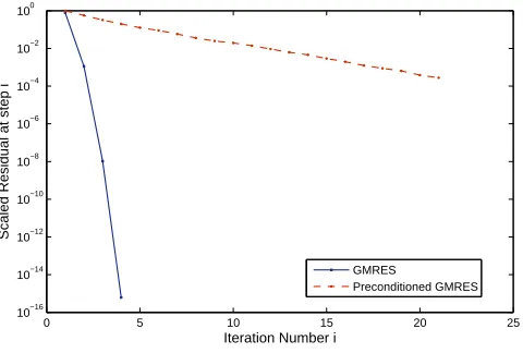
Figure 1. Convergence histories of GMRES for preconditioning technique.
0 5 10 15 20 25
10−16
10−14
10−12
10−10
10−8
10−6
10−4
10−2
100
Iteration Number i
Scaled Residual at step i
GMRES
Preconditioned GMRES
The detailed comments concerning the preconditioned GMRES algorithm (PGMRES)
can be found in [17].
3.2. Preconditioned CGN. One of the simplest methods for solving
nonsymmet-ric linear systemB(n+1)V(n+1)=b(n+1)is to apply the CG iterations to the normal
equationsB(n+1)TB(n+1)V(n+1) =B(n+1)Tb(n+1) which is called the CGN method
[16]. We note that the convergence of CGN is controlled by the eigenvalue ofB(n+1)TB(n+1).
Thus the convergence of CGN is determined by the singular value of B(n+1). Now,
suppose that the CG iterations be applied to the normal equationsB(n+1)TB(n+1)V(n+1)=
B(n+1)Tb(n+1), whereB(n+1)TB(n+1) has 2-norm condition number κ. Then the
A-norm of the errors satisfy
∥r(in+1)∥2 ∥r(0n+1)∥2
≤2(κ−1
κ+ 1)
i, (3.4)
which implies ifκis reseanblely large, convergence to a specified tolerance can be
ex-pected inO(κ) iteration. A disadvantage of the CGN method is that the convergence
rate can be slow. Therefore, preconditioner technique could be exploited to accel-erate the convergence rate of the CGN method. The preconditioned CGN (PCGN)
algorithm is given in [18].
4. Numerical Experiments
In this section, we report the results of numerical experiments to compare the performance and efficiency of preconditioned methods that introduced in the previous section.
All programs run in MATLAB R2012a. The tests have been performed on a computer with the configuration:
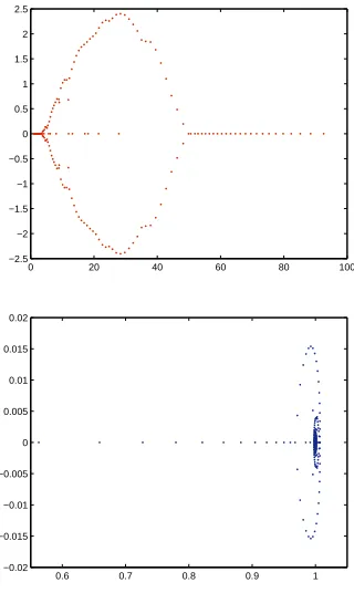
Figure 2. Left hand figure: Eigenvalues distribution of
noprecondi-tioning (J = 200, N = 200). Right hand figure: Eigenvalues
distri-bution of sparse band and diagonal preconditioning (J = 200, N =
200).
0 20 40 60 80 100 −2.5
−2 −1.5 −1 −0.5 0 0.5 1 1.5 2 2.5
0.6 0.7 0.8 0.9 1 −0.02
−0.015 −0.01 −0.005 0 0.005 0.01 0.015 0.02
Figure 3. Convergence histories of CGN for preconditioning technique.
0 20 40 60 80 100 120
10−8
10−6
10−4
10−2
100
102
104
Iteration Number i
Scaled Residual at step i
CGN
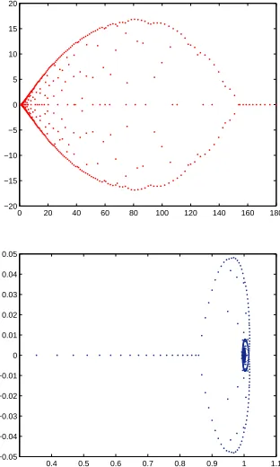
Figure 4. Left hand figure: Eigenvalues distribution of
noprecon-ditioning (J = 500,N = 500) Right hand figure: Eigenvalues
distri-bution of ILU preconditioning (luinc(B(n+1)TB(n+1),0.01),J = 500,
N = 500.
0 20 40 60 80 100 120 140 160 180 −20
−15 −10 −5 0 5 10 15 20
0.4 0.5 0.6 0.7 0.8 0.9 1 1.1 −0.05
−0.04 −0.03 −0.02 −0.01 0 0.01 0.02 0.03 0.04 0.05
• 4GB RAM memory under Windows seven
The stopping criterion is
∥r(in+1)∥2 ∥b(n+1)∥2
< ϵ, (4.1)
wherer(in+1)is the residual vector afteriiterations.
Example 1. In this example, we consider the time-independent space-fractional
convection-diffusion model with ω1 = 0.8, ϑ1 = 1.5, k(x) = x2, h(x) = −1,ϕ(x) =
x2(1−x) and
z1(x, t) = 1.815207368t
6
5x2−1.815207368t
6
5x4−2.256758334√tx4
+ 2.256758334x6√t+x2+x2t2−x4−x4t2, 0< x <1, 0< t≤1.
(4.2)
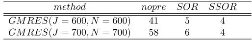
Table 1. The average number of iterations of GMRES and
precon-ditioned GMRES.
method nopre SOR SSOR
GM RES(J = 600, N= 600) 41 5 4
GM RES(J = 700, N= 700) 58 6 4
a): GMRES with band and diagonal preconditioning and without
precondition-ing (ϵ= 10−17).
Band and Diagonal Preconditioner: A simple preconditioner would be sparse band and diagonal matrix constructed by considering the special
struc-ture of the original matrix. The toolbox of MATLAB supplies a function
spdiags, that can be used to produce sparse band and diagonal
precondi-tioner. In our tests, we use
d= [−10 : 10];
C(n+1)=spdiags(B(n+1), d);
[m, m] =size(B(n+1));
M(n+1)=spdiags(C(n+1), d, m, m);
b): CGN with incomplete Cholesky preconditioning and without
precondition-ing (ϵ= 10−8).
ILU preconditioner: Incomplete LU (ILU) factorisations constitute one of the best known classes of general-purpose preconditioners. It is known that ILU preconditioners tend to cluster eigenvalues. A general ILU factorization computes a sparse approximation of the LU factorization. Incomplete LU
factorization is often used as a preconditioner (see [17]). The toolbox of
Mat-labsupplies a functionluinc, incomplete lu factorization, that can be used to
produce ILU preconditioners. The idea behindluincis simple: start a normal
LU factorization but if any entry in the factorization is small, set it to zero. In the above-mentioned example we used ILU preconditioner where:
a) Preconditioner (1): [L(n+1),U(n+1)] =luinc(B(n+1)TB(n+1),′0′) is no fill
ILU decomposition
b) Preconditioner (2): [L(n+1),U(n+1)] =luinc(B(n+1)TB(n+1), τ) is an ILU
decomposition of A with thresholdτ= 0.01.
We choose J = 200, N = 200. Figure 1 shows convergence curve corresponding to
23 steps of the GMRES and a preconditioned GMRES iterations. As Figure 1 illus-trates, the GMRES iterations for this linear system converges slowly. The condition
numbers ofB(n+1) andW(n+1) are 98.9 and 3.27, respectively, so the deterioration
in convergence can be explained by conditioning alone. When an iterative method stagnates like this, it is time to look for a better preconditioner. Distributions of the
eigenvalues of matrixB(n+1) and matrixM(n+1)−1B(n+1) are shown in Figure 2. It
Figure 5. Left hand figure: Eigenvalues distribution of
noprecondi-tioning (J = 600, N = 600). Right hand figure: Eigenvalues
distri-bution of sparse band and diagonal preconditioning (J = 600, N =
600).
0 20 40 60 80 100 120 140 160 180 200 −25
−20 −15 −10 −5 0 5 10 15 20 25
0.75 0.8 0.85 0.9 0.95 1 1.05 1.1 −0.02
−0.015 −0.01 −0.005 0 0.005 0.01 0.015 0.02
that the eigenvalues of preconditioning are clustered around 1. Therefore, one goal of preconditioning is to improve this distribution by grouping the eigenvalues into a few small clusters and around 1 as approximate as possible.
For second strategy, we choose J = 500, N = 500. The CGN algorithm, without
preconditioning, converges very badly as shown in Figure 3. This can be explained by looking to the eigenvalues. As can be seen in Figure 4, most of the eigenvalues are close to zero, which leads to a bad convergence. The eigenvalues of the ILU pre-conditioning are shown in Figure 4. The difference in convergence speed between a preconditioned matrix with eigenvalues close to 1 and an unpreconditioned matrix with the eigenvalues close to zero is shown in Figure 4.
Example 2. As second example, we consider the fractional advection-dispersion
model withω2= 0.5,ϑ2= 1.5,α1=−1,ϕ(x) =x2 and
z2(x, t) =x2+ 1.128379167
√
tx2+ 2.256758334x32 + 2.256758334x32t,
0< x <1, 0< t≤1. (4.3)
The results of the previous example show that the CGN in composition precondition-ers don’t work very well but by using GMRES method in composition preconditionprecondition-ers, we get less iteration number than CGN method. In order to solve the linear system
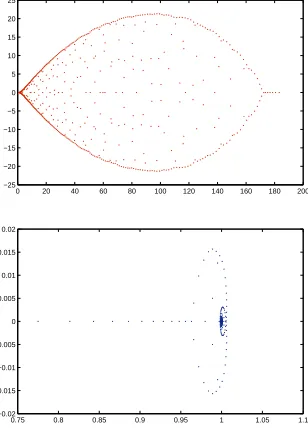
Figure 6. Left hand figure: Eigenvalues distribution of
noprecondi-tioning (J = 700, N = 700). Right hand figure: Eigenvalues
distri-bution of sparse band and diagonal preconditioning (J = 700, N =
700).
0 50 100 150 200 250
−30 −20 −10 0 10 20 30
0.7 0.75 0.8 0.85 0.9 0.95 1 1.05 −0.025
−0.02 −0.015 −0.01 −0.005 0 0.005 0.01 0.015 0.02 0.025
a: GMRES in combination of the SOR and SSOR preconditioners and without
preconditioning (ϵ= 10−7).
Preconditioner based on relaxation technique: Suppose thatB(n+1)=
D(n+1)−E(n+1)−F(n+1), in which D(n+1) is the diagonal of A, −E(n+1)
its strict lower part, and −F(n+1) its strict upper part, as was seen in [17],
the SOR and SSOR preconditioner are defined by a) SOR
Precondition-ing:M(n+1)=ω1(D(n+1)−ωE(n+1)),
b) SSOR Preconditioning:M(n+1)= ω(21−ω)(D(n+1)−ωE(n+1))D(n+1)−1(D(n+1)+
ωF(n+1)),
where ω is called the relaxation parameter. The more explanations of the
preconditioners can be found in [17].
shown in Table 1. We can see that the average number of iterations required by the preconditioned GMRES method is less than GMRES method.
5. Concluding remarks
We present two preconditioned iterative methods to solve linear systems arising from the discretization of fractional advection-diffusion equations. Numerical exper-iments confirm that the methods perform very well, easily obtaining the solution of large systems that are infeasible to solve using traditional methods.
References
[1] R. Barrett, M. Berry, T. F. Chan, J. Demmel, J. Donato, J. Dongarra, V. Eijkhout, R . Pozo, C. Romine. and H. Van der Vorst,Templates for the solution of linear systems: Building blocks for iterative methods, SIAM, 1994.
[2] D. Benson, R. Schumer, M. M. Meerschaert and S. W. Wheatcraft,Fractional dispersion, Lvy motion, and the MADE tracer tests, Transport Porous Media42(2001), 21140.
[3] D. Benson D, S. W. Wheatcraft, and M. M. Meerschaert,The fractional-order governing equa-tion of Lvy moequa-tion. Water Resour Res.,36(2000), 141323.
[4] K. Burrage, N. Hale, and D. Kay,An Efficient Implicit FEM Scheme for Fractional-in-Space ReactionDiffusion Equations, SIAM J. Sci. Comput.34(4) (2012), 21452172.
[5] M. Ekici, A. Sonmezoglu, and E. M. Zayed,A new fractional sub-equation method for solving the space-time fractional differential equations in mathematical physics, Computational Methods for Differential Equations,34(2014), 153-170.
[6] Y. Lin and C. Xu,Finite difference / spectral approximations for the time-fractional diffusion equation, Journal of Computional Physics,225(2007), 1533-1552.
[7] F. Liu, P. Zhuang, V. Anh, I. Turner and K. Burrage,Stability and convergence of the difference methods for the space-time fractional advection-diffusion equation, Applied Mathematics and Computation,191(2007), 12-20.
[8] J. Liesen and P. Tich Y,The worst-case GMRES for normal matrices, BIT, 44 (2004), 7998. [9] M. M. Meerschaert and C. Tadjeran, Finite difference approximations for fractional
advec-tiondispersion flow equations, J Comput Appl Math172(2004), 6577.
[10] M. M. Meerschaert and C. Tadjeran, Finite difference approximations for two-sided space-fractional partial differential equations, Appl Numer Math56(2006) 8090.
[11] T. Moroney and Q. Yang,A banded preconditioner for the two-sided, nonlinear space-fractional diffusion equation, Computers and Mathematics with Applications5(2013), 659-667.
[12] A. A. Neamaty, B. Agheli, and M. Adabitabar.Numerical solution for boundary value prob-lem of fractional order with approximate Integral and derivative, Computational Methods for Differential Equations3(2014) 195-204.
[13] C. C. Paige and M. A. Saunders,Solution of sparse indefinite systems of linear equations, SIAM journal on numerical analysis12(1975), 617-629.
[14] I. Podlubny,Fractional Differential Equations, Academic Press, New York, 1974.
[15] Y. Saad and M. H. Schultz, GMRES: A generalized minimal residual algorithm for solving nonsymmetric linear systems, SIAM J. Sci. Stat. Comput.7(1986) 856-869.
[16] L. N. Trefehen and D. Bau,Numerical linear algebra, SIAM, Philadelphoa, 1997. [17] Y. Saad,Iterative methods for sparse linear systems, SIAM, Philadelphoa, 2003.
[18] Y. Saad,A flexible inner-outer preconditioned gmres algorithm, SIAM J. Sci. Comput.14(2) (1993) 461469.
[19] H. Wang, K. Wang, T. Sircar,AdirectO(Nlog2N)finite difference method for fractional dif-fusion equations, Journal of Computional Physics,229(2010), 8095-8104.
[21] Q. Yang, I. Turner, F. Liu, M. Ilic ,Novel numerical methods for solving the time-space fractional diffusion equation in 2D, SIAM J. Sci. Comput.33(3) (2011), 11591180.
[22] Q. Yang, T. Moroney, K. Burrage, I. Turner, and F. Liu,Novel numerical methods for time-space fractional reaction diffusion equations in two dimensions, Aust. New Zealand Ind. Appl. Math. J.52(2011), 395409.