Adv. Radio Sci., 9, 139–143, 2011 www.adv-radio-sci.net/9/139/2011/ doi:10.5194/ars-9-139-2011
© Author(s) 2011. CC Attribution 3.0 License.
Advances in
Radio Science
Smoothing techniques for decision-directed MIMO OFDM channel
estimation
P. Beinschob and U. Z¨olzer
Department of Signal Processing and Communications, Helmut-Schmidt-Universit¨at/University of the Federal Armed Forces, Hamburg, Holstenhofweg 85, 22043 Hamburg, Germany
Abstract. With the purpose of supplying the demand of faster and more reliable communication, multiple-input multiple-output (MIMO) systems in conjunction with Or-thogonal Frequency Division Multiplexing (OFDM) are sub-ject of extensive research. Successful Decoding requires an accurate channel estimate at the receiver, which is gained ei-ther by evaluation of reference symbols which requires des-ignated resources in the transmit signal or decision-directed approaches. The latter offers a convenient way to maximize bandwidth efficiency, but it suffers from error propagation due to the dependency between the decoding of the current data symbol and the calculation of the next channel estimate. In our contribution we consider linear smoothing techniques to mitigate error propagation by the introduction of backward dependencies in the decision-based channel estimation. De-signed as a post-processing step, frame repeat requests can be lowered by applying this technique if the data is insensi-tive to latency. The problem of high memory requirements of FIR smoothing in the context of MIMO-OFDM is ad-dressed with an recursive approach that acquires minimal re-sources with virtual no performance loss. Channel estimate normalized mean square error and bit error rate (BER) per-formance evaluations are presented. For reference, a median filtering technique is presented that operates on the MIMO time-frequency grids of channel coefficients to reduce the peak-like outliers produced by wrong decisions due to un-successful decoding. Performance in terms of Bit Error Rate is compared to the proposed smoothing techniques.
Correspondence to: P. Beinschob ([email protected])
1 Introduction
MIMO OFDM systems are strong candidates for upcom-ing mobile networks. In Spatial Multiplexupcom-ing transmission modes the channel capacity increases linearly with the num-ber of transmit and receive antennas primary at the expense of higher SNR demands and algorithmic complexity in the receiver and detection algorithms (Foschini and Gans, 1998). However, there can be observed large gaps between an-alytical derived capacity statements and realized data rates with proposed receiver designs. This is particularly true for mobile scenarios. Channel estimate errors tend to decrease the achievable rates because of the limited performance of the detection algorithms operating with channel estimates (Dall’Anese et al., 2009).
To acquire channel estimates with low errors a large num-ber of reference symbols or pilots would be necessary. Ex-clusive bandwidth has to be dedicated to reference symbols and is not available for data transmission, therefore the ef-fective data rate is reduced by the amount of pilots which is not desirable. In mobile receivers the channel estimate is quickly outdated depending on the relative radial velocity to the sender (Marzetta and Hochwald, 1999). After a time duration, commonly known as the coherence time TC, the channel state must be assumed to be completely changed.
Cellular mobile networks in urban environment addition-ally experience multipath signal propagation often referred to street canyon scenarios and alike. So, Doppler shifts due to mobility vary on different propagation paths. Fading due to shadowing might occur suddenly and the channel estimation has to keep track.
The mentioned aspects and problems of mobile multi-antenna broadband communication and the consequences for the channel estimation is addressed in this paper. To mitigate influences we propose a post-processing – smoothing – algo-rithm to refine the channel estimates acquired by a decision-directed channel estimation (DDCE) and tracking algorithm.
140 P. Beinschob and U. Z¨olzer: Smoothing techniques for decision-directed MIMO OFDM channel estimation 2 P. Beinschob and U. Z¨olzer: Smoothing Techniques for Decision-Directed MIMO OFDM Channel Estimation
Source C Π
M
nT
S/P IFFT CP
Pilots ∗
CE +
Sink −1C
Π
−
1
Det FFT CP u
s[n, k] s[n, m]
ˇ
w[n, m] ˇs[n, m]
ˇr[n, m]
h[n, m]
r[n, m]
r[n, k]
r[n, k]
L
˜
H[n, k]
˜
u
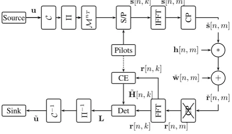
Fig. 1.MIMO-OFDM system model.
tion 2, followed by a brief review of the DDCE algorithm in Section 3. An approach to introduce linear smoothing tech-niques in the context of MIMO-OFDM channel estimation is taken in Section 4.1 and a memory-reduced version shown in Section 4.2. An alternative, non-linear filtering method is discussed in Section 4.3. Illustrating simulation results are given in Section 5 and finally a conclusion is drawn.
2 System Model and Structure
The vector of received valuesrat the time samplemof a MIMO system is the superposition ofL·nT previously sent
samples and the currentnTsamples, whereL+1is the length
of the sampled channel impulse response andnTis the
num-ber of transmit antennas. It is given by
r[m] =
L
X
l=0
h[l, m]·s[m−l] + ˜w[m], (1)
where s[m]denotes the current vector of symbols of each transmit antenna, w is an identically, independently
dis-tributed (iid) additive white Gaussian noise term andh[l, m] is the MIMO channel matrix in delay and time domain, in-dexed withlrespectivelym. The past sent samples are de-noted bys[m−l], forl 6= 0, l ≤L. The data symbols of theKsubcarriers are modulated by an inverse Fast Fourier Transform (IFFT). In simulations every value correspond-ing to a transmit antenna of the resultcorrespond-ing vectors is trans-mitted using the formula above. The data symbols itself are drawn from anM-order QAM modulation alphabetS. The mapping, denoted byM{·}, modulatesκ = log2M bits to a QAM symbol. This is done consecutively for allnT
send streams/layers. The QAM constellations are considered power-normalized to simplify notation.
In frequency domain the system model in Eq. (1) can be described as
r[n, k] =H[n, k]·s[n, k] +w[n, k], (2) wherendenotes the time index of an OFDM symbol and kits subcarrier index. The vectorsr[n, k]andw[n, k]are of dimensionnR×1,s[n, k]ofnT ×1and the matrixH[n, k]
ofnR×nT, at whichnRis the number of receive antennas.
In simulations the time domain MIMO channel coefficients hr,t[l, m], r = 1, . . . , nR, t = 1, . . . , nT are modeled
us-ing the 3GPP spatial model which was developed to evalu-ate receiver algorithms in MIMO scenarios (3rd Generation Partnership Project , 3GPP). The superposed received signals are transferred back into the frequency domain with the help of a FFT, resulting in the vectorsr[n, k]of Eq. (2). Perfect synchronization is assumed and total avoidance of block in-terference, i.e. the cyclic prefix is longer than the maximum delay path. The system’s performance is evaluated in terms of bit error rates determined from hard decided channel de-coder output. The channel dede-coder operates on soft informa-tion in form of channel log-likelihood ratios (LLRs),L. A
block diagram depicting the system model is given in Fig. 1.
3 Decision-Directed Recursive Least Squares (RLS) Channel Estimation
MIMO-RLS algorithm estimates auto- and cross-correlation matricesΦresp.θ, time adaptive with forgetting factorξas described by Kay (1993). The channel estimation is done on each subcarrierkindividually.
Φ[n, k] =ξ·Φ[n−1, k] +s[n, k]·sH[n, k] (3)
θ[n, k] =ξ·θ[n−1, k] +s[n, k]·rH[n, k] (4) An estimate of the channel matrix is obtained as follows:
˜
H[n, k] = Φ−1[n, k]·θ[n, k]H
. (5)
From the MIMO bit-wise log-likelihood ratio detection out-put, that is soft information of channel output L,
recon-structed send vectors are available. After the pilot sequence
Fig. 1. MIMO-OFDM system model.
The DDCE based on Least Squares works well with a small number of pilot symbols in quasi-static scenarios.
The paper is organized as follows. The underlying sys-tem model in time and frequency-domain is presented in Sect. 2, followed by a brief review of the DDCE algorithm in Sect. 3. An approach to introduce linear smoothing tech-niques in the context of MIMO-OFDM channel estimation is taken in Sect. 4.1 and a memory-reduced version shown in Sect. 4.2. An alternative, non-linear filtering method is dis-cussed in Sect. 4.3. Illustrating simulation results are given in Sect. 5 and finally a conclusion is drawn.
2 System model and structure
The vector of received valuesr at the time sample mof a MIMO system is the superposition ofL·nTpreviously sent samples and the currentnTsamples, whereL+1 is the length of the sampled channel impulse response andnTis the num-ber of transmit antennas. It is given by
r[m] =
L X l=0
h[l,m] ·s[m−l] + ˜w[m], (1)
wheres[m] denotes the current vector of symbols of each transmit antenna, w is an identically, independently dis-tributed (iid) additive white Gaussian noise term and h[l,m]
is the MIMO channel matrix in delay and time domain, in-dexed withl respectivelym. The past sent samples are de-noted bys[m−l], forl6=0,l≤L. The data symbols of theK subcarriers are modulated by an inverse Fast Fourier Trans-form (IFFT). In simulations every value corresponding to a transmit antenna of the resulting vectors is transmitted using the formula above. The data symbols itself are drawn from anM-order QAM modulation alphabetS. The mapping, de-noted byM{·}, modulatesκ=log2Mbits to a QAM symbol. This is done consecutively for all nT send streams/layers. The QAM constellations are considered power-normalized to simplify notation.
In frequency domain the system model in Eq. (1) can be described as
r[n,k] =H[n,k] ·s[n,k] +w[n,k], (2) wherendenotes the time index of an OFDM symbol andk its subcarrier index. The vectorsr[n,k]andw[n,k]are of dimension nR×1, s[n,k] ofnT×1 and the matrix H[n,k] of nR×nT, at which nR is the number of receive anten-nas. In simulations the time domain MIMO channel coeffi-cientshr,t[l,m], r=1,...,nR, t=1,...,nTare modeled us-ing the 3GPP spatial model which was developed to evalu-ate receiver algorithms in MIMO scenarios (3rd Generation Partnership Project , 3GPP). The superposed received signals are transferred back into the frequency domain with the help of a FFT, resulting in the vectorsr[n,k]of Eq. (2). Perfect synchronization is assumed and total avoidance of block in-terference, i.e. the cyclic prefix is longer than the maximum delay path. The system’s performance is evaluated in terms of bit error rates determined from hard decided channel de-coder output. The channel dede-coder operates on soft informa-tion in form of channel log-likelihood ratios (LLRs), L. A block diagram depicting the system model is given in Fig. 1.
3 Decision-directed Recursive Least Squares (RLS) channel estimation
MIMO-RLS algorithm estimates auto- and cross-correlation matrices8resp.θ, time adaptive with forgetting factorξ as described by Kay (1993). The channel estimation is done on each subcarrierkindividually.
8[n,k] =ξ·8[n−1,k] +s[n,k] ·sH[n,k] (3)
θ[n,k] =ξ·θ[n−1,k] +s[n,k] ·rH[n,k] (4) An estimate of the channel matrix is obtained as follows:
˜
H[n,k] =8−1[n,k] ·θ[n,k]H. (5) From the MIMO bit-wise log-likelihood ratio detection out-put, that is soft information of channel output L, recon-structed send vectors are available. After the pilot sequence of lengthNP in the preamble of the frame is processed, the reconstructed send vectors
˜
s[n] =MnT{sgn{L}}, ∀n > N
P. (6)
are used to further refine the estimate of the auto- and cross-correlation matrices thus tracking the time-variable channel, as indicated by the switch in Fig. 2 (Akhtman and Hanzo, 2007). The coherence time of the channel determines the usability of the collected samples. Old samples describing an obsolete channel state should be omitted. This is accom-plished by the introduction of the forgetting factorξ. For the sake of notational simplicity the symbols is used for pilot vectors as well as the reconstructed send vectors omitting the tilde.
P. Beinschob and U. Z¨olzer: Smoothing techniques for decision-directed MIMO OFDM channel estimationP. Beinschob and U. Z¨olzer: Smoothing Techniques for Decision-Directed MIMO OFDM Channel Estimation 1413
z−1
● (·)H ● ● (θ/Φ)H ●
pilots
Det. ● ●
●
● ●
n > NP
(·)H z−1
ξ
r[n] rH[n] θ[n] H[n]
˜s[n]
Φ[n]
ξ
Fig. 2.Signal Flow Diagram for Decision Directed RLS Channel Estimation and Tracking algorithm.
of lengthNP in the preamble of the frame is processed, the reconstructed send vectors
˜s[n] =MnT{sgn{L}}, ∀n > N
P. (6) are used to further refine the estimate of the auto- and cross-correlation matrices thus tracking the time-variable channel, as indicated by the switch in Fig. 2 (Akhtman and Hanzo, 2007). The coherence time of the channel determines the usability of the collected samples. Old samples describing an obsolete channel state should be omitted. This is accom-plished by the introduction of the forgetting factorξ. For the
sake of notational simplicity the symbolsis used for pilot
vectors as well as the reconstructed send vectors omitting the tilde.
4 Smoothing Techniques
4.1 RLS Un-rolling
Post-processing after the RLS requires access to the spatial correlation samples for each OFDM symbol and subcarrier
ˇ
Φ[n, k] =s[n, k]·sH[n, k], (7)
ˇ
θ[n, k] =s[n, k]·rH[n, k]. (8)
Considering anT ×nRMIMO OFDM system withNS OFDM symbols per frame andKsubcarriers, the dimension
of the arrays isnT×nR×K×NS.
The weighted expectation value in Eq. (3) and (4) is then
Φ[n, k] =ξ·Φ[n−1, k] + ˇΦ[n, k], (9)
θ[n, k] =ξ·θ[n−1, k] + ˇθ[n, k]. (10)
It can be re-formulated as a matrix vector-multiplication. The weighting factors are exponentially decreasing with in-creasing sample indexntherefore they constitute a lower
tri-angular matrix
Ξ=
1 0 · · ·
ξ 1 0 · · ·
ξ2 ξ 1 0 · · ·
... ... ... ... 0
ξNS−1ξNS−2ξNS−3· · · 1
. (11)
The weighting along the time dimension with the forget-ting factor matrix can be applied independently on the other dimensions
ˇ
Φ0t,r,k=Ξ·Φˇt,r,k ∀t, r, k (12) and analogue
ˇ
θ0t,r,k=Ξ·θˇr,r,k. (13) With matrices (12) and (13) the ordinary channel estimate can be calculated as well
˜
H[n, k] =Φˇ0−1[n, k]·θˇ0[n, k]H. (14)
The smoothing algorithm can be derived by minimizing the modified cost function
ˇ
J[n, k] =
NS X
˜
n=1
ξ|NS−˜n|·eH[˜n, n, k]·e[˜n, n, k] (15)
with
e[˜n, n, k] =r[˜n, k]−H˜[n, k]·s[˜n, k]. (16)
As a consequence it follows a transition for the weighting matrix to be fully occupied
Ξ0=
1 ξ ξ2 ξ3 · · ·ξNS−1
ξ 1 ξ ξ2 · · ·ξNS−2
ξ2 ξ 1 ξ · · ·ξNS−3
ξ3 ξ2 ξ 1 · · ·ξNS−4 ... ... ... ... ... ...
ξNS−1ξNS−2ξNS−3ξNS−4· · · 1
. (17)
Smoothing weighting reflecting mobility induced channel time variance and effectively doubles the number of samples available for estimating the auto- and crosscorrelation matri-ces thus lowering the estimation error. Obviously, in this for-mulation arbitrary window functions can be applied as well instead of exponentially weighting factors inΞ0. So
smooth-ing weightsmooth-ing is applied by evaluatsmooth-ing
ˇ
Φ00t,r,k=Ξ0·Φˇt,r,k, (18)
ˇ
θ00t,r,k=Ξ0·θˇt,r,k, (19) Fig. 2. Signal flow diagram for decision directed RLS channel estimation and tracking algorithm.
4 Smoothing techniques
4.1 RLS un-rolling
Post-processing after the RLS requires access to the spatial correlation samples for each OFDM symbol and subcarrier
ˇ
8[n,k] =s[n,k] ·sH[n,k], (7)
ˇ
θ[n,k] =s[n,k] ·rH[n,k]. (8) Considering a nT×nR MIMO OFDM system with NS OFDM symbols per frame andKsubcarriers, the dimension of the arrays isnT×nR×K×NS.
The weighted expectation value in Eqs. (3) and (4) is then
8[n,k] =ξ·8[n−1,k] + ˇ8[n,k], (9)
θ[n,k] =ξ·θ[n−1,k] + ˇθ[n,k]. (10) It can be re-formulated as a matrix vector-multiplication. The weighting factors are exponentially decreasing with increas-ing sample indexntherefore they constitute a lower triangu-lar matrix
4=
1 0 ···
ξ 1 0 ···
ξ2 ξ 1 0 ···
..
. ... ... . .. 0 ξNS−1ξNS−2ξNS−3 ··· 1
. (11)
The weighting along the time dimension with the forgetting factor matrix can be applied independently on the other di-mensions
ˇ
80t,r,k=4· ˇ8t,r,k ∀t,r,k (12) and analogue
ˇ
θ0t,r,k=4· ˇθr,r,k. (13) With matrices (12) and (13) the ordinary channel estimate can be calculated as well
˜
H[n,k] =8ˇ0−1[n,k] · ˇθ0[n,k]
H
. (14)
The smoothing algorithm can be derived by minimizing the modified cost function
ˇ
J[n,k] =
NS
X ˜ n=1
ξ|NS− ˜n|·eH[ ˜n,n,k] ·e[ ˜n,n,k] (15)
with
e[ ˜n,n,k] =r[ ˜n,k] − ˜H[n,k] ·s[ ˜n,k]. (16) As a consequence it follows a transition for the weighting matrix to be fully occupied
40=
1 ξ ξ2 ξ3 ··· ξNS−1
ξ 1 ξ ξ2 ··· ξNS−2
ξ2 ξ 1 ξ ··· ξNS−3
ξ3 ξ2 ξ 1 ··· ξNS−4
..
. ... ... ... . .. ... ξNS−1ξNS−2ξNS−3ξNS−4 ··· 1
. (17)
Smoothing weighting reflecting mobility induced channel time variance and effectively doubles the number of sam-ples available for estimating the auto- and crosscorrelation matrices thus lowering the estimation error. Obviously, in this formulation arbitrary window functions can be applied as well instead of exponentially weighting factors in40. So smoothing weighting is applied by evaluating
ˇ
800t,r,k=40· ˇ8t,r,k, (18)
ˇ
θ00t,r,k=40· ˇθt,r,k, (19) The smoothed channel estimate for the unrolling (U) is yielded by
˜
HUS[n,k] =8ˇ00−1[n,k] · ˇθ00[n,k]H. (20) 4.2 Recursive smoothing
The unrolling approach consumes a huge amount of mem-ory impeding practical receiver implementations. Therefore a reduction of memory requirements is desirable. It is possi-ble to reformulate the algorithm again into a recursive form (Kashima et al., 2006). Defining
142 P. Beinschob and U. Z¨olzer: Smoothing techniques for decision-directed MIMO OFDM channel estimation 4 P. Beinschob and U. Z¨olzer: Smoothing Techniques for Decision-Directed MIMO OFDM Channel Estimation
Pilots nR ˇ r CP FFT Channel-Est. MIMO-Detector Smoothing MIMO-Detector Π−1
C−1 sink
r[k] ˜
s[k]
r[k]
r[k]
ˇ
Φ,θˇ
˜
H
˜
HS LD1
LA2 LD2
˜
u
Fig. 3.Receiver structure with post processing of channel estimation with discussed Smoothing techniques.
The smoothed channel estimate for the unrolling (U) is yielded by
˜
HUS[n, k] =Φˇ00−1[n, k]·θˇ00[n, k]H. (20)
4.2 Recursive Smoothing
The unrolling approach consumes a huge amount of mem-ory impeding practical receiver implementations. Therefore a reduction of memory requirements is desirable. It is possi-ble to reformulate the algorithm again into a recursive form (Kashima et al., 2006). Defining
ΦS[n, k] = NS X
˜
n=1
ξ|NS−n˜|·s[˜n, k]·sH[˜n, k], (21)
θS[n, k] = NS X
˜
n=1
ξ|NS−n˜|·s[˜n, k]·rH[˜n, k], (22)
it is possible to calculate the smoothed inverse autocorrela-tion matrixPS=Φ−S1recursive using the already estimated
inverse autocorrelation matrixΦ,
PS[n, k] =P[n, k] +ξ2·
PS[n+ 1, k]−ξ−1·P[n, k]
.
(23) So a smoothed channel estimate can also be calculated using the previously estimated channel estimateH˜ by evaluating
˜
HRS[n, k] = ˜H[n, k] +ξ·[ ˜HS[n+ 1, k]−H˜[n, k]], (24)
where n = NS, . . . ,1 and it is initialized by setting ˜
HS[NS, k] = ˜H[NS, k].
4.3 Time-Frequency Median Filtering
Decision-directed channel estimation is prone to error prop-agation and wrong decisions may lead to impulse-like out-liers in the channel estimate. As median filtering is especially suited for impulse noise it is investigated in this context as an alternative to the above discussed approaches to smoothing.
This non-linear filtering is applied on thenT ·nR
time-frequency grids resp. time-variant channel transfer functions. An important parameter is the filter kernel size. Often used sizes in image processing are3×3,5×5or7×7samples. The optimal kernel size depends on the coherence time and coherence bandwidth respectively subcarriers.
10-2
10-1
100
101
9 12 15
N
M
SE
SNR in dB ■ ■ ■ ● ● ● ▲ ▲ ▲ ◆ ◆ ◆
■ ■ 3×3
● ● 5×5 ▲ ▲ 7×7 ◆ ◆w/o Median
Fig. 4.NMSE comparison of different kernel sizes for Median
Fil-tering in a time-variable channel with simulated mobile terminal velocity of 10 m/s.
10-3
10-2
10-1
100
101
3 6 9 12 15
N
M
SE
SNR in dB ■ ■ ■ ■ ■ ■ ■ ■ ■ ■ ■ ■ ■ ● ● ● ● ● ● ● ● ● ● ● ● ● ● ● ● RLS unrolling recurs. smoothing median filter
■ ■ 3 m/s ● ● 30 m/s
Fig. 5. Decreasing averaged Normalized Mean Squared Error
(NMSE) of channel estimates for increasing SNR.
5 Simulation Results
The comparative simulations were conducted using a4×4
MIMO-OFDM system configuration withK = 128
subcar-riers and a cyclic prefix lengthL= 6and two velocity set-ups (3 m/s and 30 m/s). For a realistic channel the 3GPP
Spatial Channel Model was used with time-variant impulse responses. Uniformly distributed bits were coded using an ir-regular LDPC code with design code rate of1/2, interleaved and 4-QAM modulated. LDPC codes are chosen because of high codeword distance and parallelisable decoder struc-Fig. 3. Receiver structure with post processing of channel estimation with discussed smoothing techniques.
4
P. Beinschob and U. Z¨olzer: Smoothing Techniques for Decision-Directed MIMO OFDM Channel Estimation
Pilots
n
Rˇ
r
CP
FFT
Channel-Est.
MIMO-Detector
Smoothing
MIMO-Detector
Π
−1C
−1sink
r
[
k
]
˜
s
[
k
]
r
[
k
]
r
[
k
]
ˇ
Φ
,
θ
ˇ
˜
H
˜
H
SL
D1L
A2L
D2˜
u
Fig. 3.
Receiver structure with post processing of channel estimation with discussed Smoothing techniques.
The smoothed channel estimate for the unrolling (U) is
yielded by
˜
H
US[
n, k
] =
Φ
ˇ
00−1[
n, k
]
·
ˇ
θ
00[
n, k
]
H.
(20)
4.2 Recursive Smoothing
The unrolling approach consumes a huge amount of
mem-ory impeding practical receiver implementations. Therefore
a reduction of memory requirements is desirable. It is
possi-ble to reformulate the algorithm again into a recursive form
(Kashima et al., 2006). Defining
Φ
S[
n, k
] =
NS
X
˜ n=1
ξ
|NS−n˜|·
s
[˜
n, k
]
·
s
H[˜
n, k
]
,
(21)
θ
S[
n, k
] =
NS
X
˜
n=1
ξ
|NS−n˜|·
s
[˜
n, k
]
·
r
H[˜
n, k
]
,
(22)
it is possible to calculate the smoothed inverse
autocorrela-tion matrix
P
S=
Φ
−S1recursive using the already estimated
inverse autocorrelation matrix
Φ
,
P
S[
n, k
] =
P
[
n, k
] +
ξ
2·
P
S[
n
+ 1
, k
]
−
ξ
−1·
P
[
n, k
]
.
(23)
So a smoothed channel estimate can also be calculated using
the previously estimated channel estimate
H
˜
by evaluating
˜
H
RS[
n, k
] = ˜
H
[
n, k
] +
ξ
·
[ ˜
H
S[
n
+ 1
, k
]
−
H
˜
[
n, k
]]
,
(24)
where
n
=
N
S, . . . ,
1
and it is initialized by setting
˜
H
S[
NS
, k
] = ˜
H
[
NS
, k
]
.
4.3 Time-Frequency Median Filtering
Decision-directed channel estimation is prone to error
prop-agation and wrong decisions may lead to impulse-like
out-liers in the channel estimate. As median filtering is especially
suited for impulse noise it is investigated in this context as an
alternative to the above discussed approaches to smoothing.
This non-linear filtering is applied on the
n
T·
n
Rtime-frequency grids resp. time-variant channel transfer functions.
An important parameter is the filter kernel size. Often used
sizes in image processing are
3
×
3
,
5
×
5
or
7
×
7
samples.
The optimal kernel size depends on the coherence time and
coherence bandwidth respectively subcarriers.
10
-210
-110
010
19
12
15
N
M
SE
SNR in dB
■ ■ ■ ● ● ● ▲ ▲ ▲ ◆ ◆ ◆ ■ ■ 3×3
● ● 5×5 ▲ ▲ 7×7
◆ ◆w/o Median
Fig. 4.
NMSE comparison of different kernel sizes for Median
Fil-tering in a time-variable channel with simulated mobile terminal
velocity of 10 m
/
s.
10
-310
-210
-110
010
13
6
9
12
15
N
M
SE
SNR in dB
■ ■ ■ ■ ■ ■ ■ ■ ■ ■ ■ ■ ■ ● ● ● ● ● ● ● ● ● ● ● ● ● ● ● ● RLS unrolling recurs. smoothing median filter
■ ■ 3 m/s ● ● 30 m/s
Fig. 5.
Decreasing averaged Normalized Mean Squared Error
(NMSE) of channel estimates for increasing SNR.
5
Simulation Results
The comparative simulations were conducted using a
4
×
4
MIMO-OFDM system configuration with
K
= 128
subcar-riers and a cyclic prefix length
L
= 6
and two velocity
set-ups (3 m
/
s and 30 m
/
s). For a realistic channel the 3GPP
Spatial Channel Model was used with time-variant impulse
responses. Uniformly distributed bits were coded using an
ir-regular LDPC code with design code rate of
1
/
2
, interleaved
and
4
-QAM modulated. LDPC codes are chosen because
of high codeword distance and parallelisable decoder
struc-Fig. 4. NMSE comparison of different kernel sizes for Median
Fil-tering in a time-variable channel with simulated mobile terminal velocity of 10 m s−1.
8S[n,k] = NS X ˜ n=1
ξ|NS− ˜n|·s[ ˜n,k] ·sH[ ˜n,k], (21)
θS[n,k] = NS X ˜ n=1
ξ|NS− ˜n|·s[ ˜n,k] ·rH[ ˜n,k], (22)
it is possible to calculate the smoothed inverse autocorrela-tion matrix PS=8−S1 recursive using the already estimated inverse autocorrelation matrix8,
PS[n,k] =P[n,k] +ξ2·hPS[n+1,k] −ξ−1·P[n,k]i. (23) So a smoothed channel estimate can also be calculated using the previously estimated channel estimateH by evaluating˜
˜
HRS[n,k] = ˜H[n,k] +ξ· [ ˜HS[n+1,k] − ˜H[n,k]], (24) where n =NS,...,1 and it is initialized by setting
˜
HS[NS,k] = ˜H[NS,k].
4.3 Time-frequency median filtering
Decision-directed channel estimation is prone to error prop-agation and wrong decisions may lead to impulse-like out-liers in the channel estimate. As median filtering is especially suited for impulse noise it is investigated in this context as an alternative to the above discussed approaches to smoothing.
4
P. Beinschob and U. Z¨olzer: Smoothing Techniques for Decision-Directed MIMO OFDM Channel Estimation
Pilots
n
Rˇ
r
CP
FFT
Channel-Est.
MIMO-Detector
Smoothing
MIMO-Detector
Π
−1C
−1sink
r
[
k
]
˜
s
[
k
]
r
[
k
]
r
[
k
]
ˇ
Φ
,
θ
ˇ
˜
H
˜
H
SL
D1L
A2L
D2˜
u
Fig. 3.
Receiver structure with post processing of channel estimation with discussed Smoothing techniques.
The smoothed channel estimate for the unrolling (U) is
yielded by
˜
H
US[
n, k
] =
Φ
ˇ
00−1[
n, k
]
·
θ
ˇ
00[
n, k
]
H.
(20)
4.2 Recursive Smoothing
The unrolling approach consumes a huge amount of
mem-ory impeding practical receiver implementations. Therefore
a reduction of memory requirements is desirable. It is
possi-ble to reformulate the algorithm again into a recursive form
(Kashima et al., 2006). Defining
Φ
S[
n, k
] =
NS
X
˜ n=1
ξ
|NS−n˜|·
s
[˜
n, k
]
·
s
H[˜
n, k
]
,
(21)
θ
S[
n, k
] =
NS
X
˜ n=1
ξ
|NS−n˜|·
s
[˜
n, k
]
·
r
H[˜
n, k
]
,
(22)
it is possible to calculate the smoothed inverse
autocorrela-tion matrix
P
S=
Φ
−S1recursive using the already estimated
inverse autocorrelation matrix
Φ
,
P
S[
n, k
] =
P
[
n, k
] +
ξ
2·
P
S[
n
+ 1
, k
]
−
ξ
−1·
P
[
n, k
]
.
(23)
So a smoothed channel estimate can also be calculated using
the previously estimated channel estimate
H
˜
by evaluating
˜
H
RS[
n, k
] = ˜
H
[
n, k
] +
ξ
·
[ ˜
H
S[
n
+ 1
, k
]
−
H
˜
[
n, k
]]
,
(24)
where
n
=
N
S, . . . ,
1
and it is initialized by setting
˜
H
S[
N
S, k
] = ˜
H
[
N
S, k
]
.
4.3 Time-Frequency Median Filtering
Decision-directed channel estimation is prone to error
prop-agation and wrong decisions may lead to impulse-like
out-liers in the channel estimate. As median filtering is especially
suited for impulse noise it is investigated in this context as an
alternative to the above discussed approaches to smoothing.
This non-linear filtering is applied on the
n
T·
n
Rtime-frequency grids resp. time-variant channel transfer functions.
An important parameter is the filter kernel size. Often used
sizes in image processing are
3
×
3
,
5
×
5
or
7
×
7
samples.
The optimal kernel size depends on the coherence time and
coherence bandwidth respectively subcarriers.
10
-210
-110
010
19
12
15
N
M
SE
SNR in dB
■ ■ ■ ● ● ● ▲ ▲ ▲ ◆ ◆ ◆ ■ ■ 3×3
● ● 5×5 ▲ ▲ 7×7
◆ ◆w/o Median
Fig. 4.
NMSE comparison of different kernel sizes for Median
Fil-tering in a time-variable channel with simulated mobile terminal
velocity of 10 m
/
s.
10
-310
-210
-110
010
13
6
9
12
15
N
M
SE
SNR in dB
■ ■ ■ ■ ■ ■ ■ ■ ■ ■ ■ ■ ■ ● ● ● ● ● ● ● ● ● ● ● ● ● ● ● ● RLS unrolling recurs. smoothing median filter
■ ■ 3 m/s
● ● 30 m/s
Fig. 5.
Decreasing averaged Normalized Mean Squared Error
(NMSE) of channel estimates for increasing SNR.
5
Simulation Results
The comparative simulations were conducted using a
4
×
4
MIMO-OFDM system configuration with
K
= 128
subcar-riers and a cyclic prefix length
L
= 6
and two velocity
set-ups (3 m
/
s and 30 m
/
s). For a realistic channel the 3GPP
Spatial Channel Model was used with time-variant impulse
responses. Uniformly distributed bits were coded using an
ir-regular LDPC code with design code rate of
1
/
2
, interleaved
and
4
-QAM modulated. LDPC codes are chosen because
of high codeword distance and parallelisable decoder
struc-Fig. 5. NMSE comparison of different kernel sizes for Median
Fil-tering in a time-variable channel with simulated mobile terminal velocity of 10 m s−1.
This non-linear filtering is applied on the nT·nR time-frequency grids resp. time-variant channel transfer functions. An important parameter is the filter kernel size. Often used sizes in image processing are 3×3, 5×5 or 7×7 samples. The optimal kernel size depends on the coherence time and coherence bandwidth respectively subcarriers.
5 Simulation results
The comparative simulations were conducted using a 4×4 MIMO-OFDM system configuration withK=128 subcar-riers and a cyclic prefix lengthL=6 and two velocity set-ups (3 m s−1and 30 m s−1). For a realistic channel the 3GPP Spatial Channel Model was used with time-variant impulse responses. Uniformly distributed bits were coded using an ir-regular LDPC code with design code rate of 1/2, interleaved and 4-QAM modulated. LDPC codes are chosen because of high codeword distance and parallelisable decoder struc-ture (Richardson et al., 2001). They are also employed in the IEEE 802.11n Standard for MIMO systems.
P. Beinschob and U. Z¨olzer: Smoothing techniques for decision-directed MIMO OFDM channel estimation 143
P. Beinschob and U. Z¨olzer: Smoothing Techniques for Decision-Directed MIMO OFDM Channel Estimation
5
10
-710
-610
-510
-410
-310
-210
-110
03
6
9
12
15
B
E
R
SNR in dB
■ ■
■
■
■ ■
■
■
■ ■
■
■
■
● ● ●
●
●
● ● ●
●
●
● ● ●
●
● RLS unrolling
recurs. smoothing median filter
■ ■ 3 m/s
● ● 30 m/s
Fig. 6.
Comparison of Bit Error Rates for discussed smoothing
tech-niques.
ture (Richardson et al., 2001). They are also employed in the
IEEE 802.11n Standard for MIMO systems.
For different median kernel sizes simulations had been
conducted and the results in terms of NMSE are depicted
in Fig. 4. A kernel size of
5
×
5
resulted in lowest average
channel estimation errors which was then used in the overall
comparative simulations.
Results in terms of channel estimation error measured in
normalised mean squared error (NMSE) are presented in
Fig. 5. A turbo-like cliff region (ten Brink, 2000) around
9 dB was observed. For SNR below this threshold the
de-tector could not reproduce the send vectors reliable therefore
error propagation in the decision-directed channel estimation
algorithm started rendering complete frames useless and
fi-nally resulting in high channel estimation errors. Above the
identified threshold the NMSE dramatically decreased. In
this region performance differences for Median filtering are
visible, whereas for the unrolling and the recursive
Smooth-ing there were no significant differences in performance
ob-servable – the curves are almost identical, slightly better for
the unrolling approach.
The Bit Error Rate (BER) versus SNR are depicted in
Fig. 6. The results reflect the same tendency as the NMSE
results did. In comparison to the linear smoothing techniques
the performance of the Median filter is worse.
Reliable transmission is possible in the slowly time-variant
case above 10 dB SNR employing one of the linear
smooth-ing methods. It needs 12 dB or more with the Median
filter-ing method. However, for the higher velocity the difference
in minimum SNR is insignificant due to the high impact of
intercarrier interference.
6
Conclusions
In this paper we have discussed smoothing techniques in the
context of MIMO OFDM channel estimation. The output
of a bandwidth-efficient decision-directed channel
estima-tion and tracking algorithm is post-processed to improve the
estimate’s accuracy in mobile scenarios by effectively
dou-bling the number of samples available for correlation matrix
estimation. In a first approach, the modification of the RLS
algorithm leads to a smoothing with high memory
require-ments. A memory efficient recursive smoothing algorithm
has been presented having virtually no loss in NMSE or BER
performance compared to the first approach in the conducted
simulations with two velocity scenarios. As an alternative,
median filtering is compared to the above mentioned. While
it leads to comparable results for the high velocity case, a gap
for the lower one reveals the disadvantage of the static kernel
size in this method.
However, in future work these results has to be verified
with measurement setups. Nevertheless the simulations
in-dicate a potential to post-processing algorithms if the
trans-mitted data is not sensitive to delays caused by the increased
processing time and latency.
References
3rd Generation Partnership Project (3GPP): Spatial channel model
for Multiple Input Multiple Output (MIMO) simulations, Tech.
Spec. Group Radio Access Network, Tech. Report 25.996, Rel.
8.0.0, 2008.
Akhtman, J. and Hanzo, L.: Advanced Channel Estimation for
MIMO-OFDM in Realistic Channel Conditions, IEEE
Interna-tional Conference on Communications, ICC ’07, pp. 2528–2533,
doi:10.1109/ICC.2007.418, 2007.
Dall’Anese, E., Assalini, A., and Pupolin, S.: On the Effect of
Imperfect Channel Estimation upon the Capacity of Correlated
MIMO Fading Channels, pp. 1–5, doi:10.1109/VETECS.2009.
5073728, 2009.
Foschini, G. J. and Gans, M. J.: On Limits of Wireless
Communi-cations in a Fading Environment when Using Multiple Antennas,
Wireless Personal Communications: An International Journal, 6,
311–335, 1998.
Kashima, T., Fukawa, K., and Suzuki, H.: Recursive Least Squares
Channel Estimator with Smoothing and Removing for
Iterative-MAP Receiver of MIMO-OFDM Mobile Communications, 7,
3052–3057, doi:10.1109/ICC.2006.255273, 2006.
Kay, S. M.: Estimation Theory, Fundamentals of statistical signal
processing, vol. 1, Prentice Hall PTR, Upper Saddle River, NJ,
1993.
Marzetta, T. and Hochwald, B.: Capacity of a mobile
multiple-antenna communication link in Rayleigh flat fading, IEEE
Trans-actions on Information Theory, 45, 139–157, doi:10.1109/18.
746779, 1999.
Richardson, T. J., Shokrollahi, M. A., and Urbanke, R. L.: Design of
capacity-approaching irregular low-density parity-check codes,
IEEE Trans. Inf. Theory, 47, 619–637, doi:http://dx.doi.org/10.
1109/18.910578, 2001.
ten Brink, S.: Designing Iterative Decoding Schemes with the
Ex-trinsic Information Transfer Chart, AEU Int. J. Electron.
Com-mun., pp. 389–398, 2000.
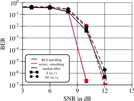
Fig. 6. Comparison of Bit Error Rates for discussed smoothing
tech-niques.
For different median kernel sizes simulations had been conducted and the results in terms of NMSE are depicted in Fig. 4. A kernel size of 5×5 resulted in lowest average channel estimation errors which was then used in the overall comparative simulations.
Results in terms of channel estimation error measured in normalised mean squared error (NMSE) are presented in Fig. 5. A turbo-like cliff region (ten Brink, 2000) around 9 dB was observed. For SNR below this threshold the de-tector could not reproduce the send vectors reliable therefore error propagation in the decision-directed channel estimation algorithm started rendering complete frames useless and fi-nally resulting in high channel estimation errors. Above the identified threshold the NMSE dramatically decreased. In this region performance differences for Median filtering are visible, whereas for the unrolling and the recursive Smooth-ing there were no significant differences in performance ob-servable – the curves are almost identical, slightly better for the unrolling approach.
The Bit Error Rate (BER) versus SNR are depicted in Fig. 6. The results reflect the same tendency as the NMSE results did. In comparison to the linear smoothing techniques the performance of the Median filter is worse.
Reliable transmission is possible in the slowly time-variant case above 10 dB SNR employing one of the linear smooth-ing methods. It needs 12 dB or more with the Median filter-ing method. However, for the higher velocity the difference in minimum SNR is insignificant due to the high impact of intercarrier interference.
6 Conclusions
In this paper we have discussed smoothing techniques in the context of MIMO OFDM channel estimation. The output
of a bandwidth-efficient decision-directed channel estima-tion and tracking algorithm is post-processed to improve the estimate’s accuracy in mobile scenarios by effectively dou-bling the number of samples available for correlation matrix estimation. In a first approach, the modification of the RLS algorithm leads to a smoothing with high memory require-ments. A memory efficient recursive smoothing algorithm has been presented having virtually no loss in NMSE or BER performance compared to the first approach in the conducted simulations with two velocity scenarios. As an alternative, median filtering is compared to the above mentioned. While it leads to comparable results for the high velocity case, a gap for the lower one reveals the disadvantage of the static kernel size in this method.
However, in future work these results has to be verified with measurement setups. Nevertheless the simulations in-dicate a potential to post-processing algorithms if the trans-mitted data is not sensitive to delays caused by the increased processing time and latency.
References
3rd Generation Partnership Project (3GPP): Spatial channel model for Multiple Input Multiple Output (MIMO) simulations, Tech. Spec. Group Radio Access Network, Tech. Report 25.996, Rel. 8.0.0, 2008.
Akhtman, J. and Hanzo, L.: Advanced Channel Estimation for MIMO-OFDM in Realistic Channel Conditions, IEEE Interna-tional Conference on Communications, ICC ’07, pp. 2528–2533, doi:10.1109/ICC.2007.418, 2007.
Dall’Anese, E., Assalini, A., and Pupolin, S.: On the Effect of Imperfect Channel Estimation upon the Capacity of Correlated MIMO Fading Channels, pp. 1–5, doi:10.1109/VETECS.2009. 5073728, 2009.
Foschini, G. J. and Gans, M. J.: On Limits of Wireless Communi-cations in a Fading Environment when Using Multiple Antennas, Wireless Personal Communications: An International Journal, 6, 311–335, 1998.
Kashima, T., Fukawa, K., and Suzuki, H.: Recursive Least Squares Channel Estimator with Smoothing and Removing for Iterative-MAP Receiver of MIMO-OFDM Mobile Communications, 7, 3052–3057, doi:10.1109/ICC.2006.255273, 2006.
Kay, S. M.: Estimation Theory, Fundamentals of statistical signal processing, vol. 1, Prentice Hall PTR, Upper Saddle River, NJ, 1993.
Marzetta, T. and Hochwald, B.: Capacity of a mobile multiple-antenna communication link in Rayleigh flat fading, IEEE Trans-actions on Information Theory, 45, 139–157, doi:10.1109/18. 746779, 1999.
Richardson, T. J., Shokrollahi, M. A., and Urbanke, R. L.: Design of capacity-approaching irregular low-density parity-check codes, IEEE Trans. Inf. Theory, 47, 619–637, doi:http://dx.doi.org/10. 1109/18.910578, 2001.
ten Brink, S.: Designing Iterative Decoding Schemes with the Ex-trinsic Information Transfer Chart, AEU Int. J. Electron. Com-mun., pp. 389–398, 2000.