The Thirty-Third AAAI Conference on Artificial Intelligence (AAAI-19)
Convex Formulations for Fair Principal Component Analysis
Matt Olfat,
1Anil Aswani
1 1UC BerkeleyBerkeley, CA 94720
[email protected], [email protected]
Abstract
Though there is a growing literature on fairness for supervised learning, incorporating fairness into unsupervised learning has been less well-studied. This paper studies fairness in the context of principal component analysis (PCA). We first define fairness for dimensionality reduction, and our definition can be interpreted as saying a reduction is fair if information about a protected class (e.g., race or gender) cannot be inferred from the dimensionality-reduced data points. Next, we develop convex optimization formulations that can improve the fairness (with respect to our definition) of PCA and kernel PCA. These formulations are semidefinite programs, and we demonstrate their effectiveness using several datasets. We conclude by showing how our approach can be used to perform a fair (with respect to age) clustering of health data that may be used to set health insurance rates.
1
Introduction
Despite the success of machine learning in informing policies and automating decision-making, there is growing concern about the fairness (with respect to protected classes like race or gender) of the resulting policies and decisions (Miller 2015; Rudin 2013; Angwin et al. 2016; Munoz, Smith, and Patil 2016). Hence, several groups have studied how to define fairness for supervised learning (Hardt, Price, and Srebro 2016; Calders, Kamiran, and Pechenizkiy 2009; Dwork et al. 2012; Zliobaite 2015) and developed supervised learners that maintain high prediction accuracy while reducing unfairness (Berk et al. 2017; Chouldechova 2017; Hardt, Price, and Srebro 2016; Zafar et al. 2017; Olfat and Aswani 2017).
However, fairness in the context of unsupervised learning has not been well-studied to date. One reason is that fairness is easier to define in the supervised setting, where positive predictions can often be mapped to positive decisions (e.g., an individual who is predicted to not default on a loan maps to the individual being offered a loan). Such notions of fairness cannot be used for unsupervised learning, which does not involve making predictions. A second reason is that it is not obvious why fairness is an issue of relevance to unsupervised learning, since predictions are not made.
Copyright c2019, Association for the Advancement of Artificial Intelligence (www.aaai.org). All rights reserved.
1.1
Relevance of fairness to unsupervised
learning
Fairness is important to unsupervised learning: First, unsuper-vised learning is often used to generate qualitative insights from data. Examples include visualizing high-dimensional data through dimensionality-reduction and clustering data to identify common trends or behaviors. If such qualitative insights are used to generate policies, then there is an oppor-tunity to introduce unfairness in the resulting policies if the results of the unsupervised learning are unequal for different protected classes (e.g., race or gender). We present such an example in Section 6 using individual health data.
Second, unsupervised learning is often useSd as a pre-processing step for other learning methods. For instance, dimensionality reduction is sometimes performed prior to clustering, and hence fair dimensionality reduction could in-directly provide methods for fair clustering. Similarly, there are no fairness-enhancing versions of most supervised learn-ers. Consequently, techniques for fair unsupervised learning could be combined with state-of-the-art supervised learners to develop new fair supervised learners. In fact, the past work most related to this paper concerns techniques that have been developed to generate fair data transformations that main-taining high prediction accuracy for classifiers that make predictions using the transformed data (Dwork et al. 2012; Zemel et al. 2013; Feldman et al. 2015); however, these past works are most accurately classified as supervised learning because the data transformations are computed with respect to a label used for predictions.
clustering techniques. Finally, a series of work has emerged using auto-encoders in the the context of deep classifica-tion. This area is promising, but suffers from a lack of the-oretical guarantees and is further oriented almost entirely around an explicit classification task (Beutel et al. 2017; Zhang, Lemoine, and Mitchell 2018). In contrast, our method has applications in both supervised and unsupervised learning tasks, and well-defined convergence and optimality guaran-tees.
1.2
Outline and novel contributions
This paper studies fairness for principal component analysis (PCA), and we make three main contributions: First, in Sec-tion 3 we propose and motivate a novel quantitative definiSec-tion of fairness for dimensionality reduction. Second, in Section 5 we develop convex optimization formulations for fair PCA and fair kernel PCA. Third, in Section 6 we demonstrate the efficacy of our semidefinite programming (SDP) formu-lations using several datasets, including using fair PCA as preprocessing to perform fair (with respect to age) clustering of health data that can impact health insurance rates.
2
Notation
Let[n] ={1, . . . , n},1(u)be the Heaviside function, and let ebe the vector whose entries are all 1. A positive semidefinite matrixU with dimensionsq×q is denotedU ∈ Sq+ (or U 0when dimensions are clear). We use the notationh·,·i to denote the inner product andIthe identity matrix.
Our data consists of 2-tuples (xi, zi)fori = 1, . . . , n, wherexi∈Rpare a set of features, andzi∈ {−1,1}label a protected class. For a matrixW, thei-th row ofWis denoted Wi. Let X ∈ Rn×p andZ ∈ Rn be the matrices so that Xi = (xi−x)T andZi = zi, wherex= n1Pixi. Also, we use the notationΠ :Rp→Rdto refer to a function that performs dimensionality reduction on thexidata, wheredis the dimension of the dimensionality-reduced data.
Let P = {i : zi = +1} be the set of indices where the protected class is positive, and similarly letN = {i : zi =−1}be the set of indices where the protected class is negative. We use#P and#N for the cardinality of these sets. Furthermore, we defineX+to be the matrix whose rows arexTi fori∈P, and we similarly defineX−to be the matrix whose rows arexTi fori∈N. Next, letΣ+b andΣb− be the sample covariances matrices ofX+andX−, respectively.
For a kernel functionk:Rp×Rp→R+, letK(X, X0) = [k(Xi, Xj0)]ijbe the transformed Gram matrix. Since the ker-nel trickinvolves replacingxTixjwithK(xi, xj), the benefit of the above notation is it allows us to replaceX(X0)Twith
K(X, X0)as part of applying the kernel trick.
3
Fairness for dimensionality reduction
Definitions of fairness for supervised learning (Hardt, Price, and Srebro 2016; Dwork et al. 2012; Calders, Kamiran, and Pechenizkiy 2009; Zliobaite 2015; Feldman et al. 2015; Chouldechova 2017; Berk et al. 2017) specify that predic-tions conditioned on the protected class are roughly equiv-alent. However, these fairness notions cannot be used fordimensionality reduction because predictions are not made in unsupervised learning. This section discusses fairness for dimensionality reduction. We first provide and motivate a general quantitative definition of fairness, and then present several important cases of this definition.
3.1
General definition
Consider a fixed classifierh(u, t) :Rd×R→ {−1,+1}that inputs featuresu∈ Rdand a thresholdt, and predicts the protected classz∈ {−1,+1}. We say that a dimensionality reductionΠ :Rp→Rdis∆(h)-fair if
P
h(Π(x), t) = +1z= +1
−Ph(Π(x), t) = +1z=−1
≤∆(h), ∀t∈R. (1)
Moreover, letFbe a family of classifiers. Then we say that a dimensionality reductionΠ :Rp→
Rdis∆(F)-fair if it is
∆(h)-fair for all classifiersh∈ F.
Our fairness definition can be interpreted via classifica-tion: Observe that the first term in the left-hand-side of (1) is the true positive rate of the classifierhin predicting the protected class using the dimensionality-reduced variable Π(x)at thresholdt, and the second term is the corresponding false positive rate. Thus,∆(h)in our definition (1) can be interpreted as bounding the accuracy of the classifierhin pre-dicting the protected class using the dimensionality-reduced variableΠ(x).
Note that eq. (1) is analogous todisparate impactfor clas-sifiers (Calders, Kamiran, and Pechenizkiy 2009; Feldman et al. 2015), where we require that treatment not vary at all between protected classes. This has often been criticized as too strict of a notion in classification, and so alternate notions of fairness have been developed, such asequalized oddsandequalized opportunity(Hardt, Price, and Srebro 2016). Instead of equalizing all treatment across protected classes, these notions instead focus on equalizing error rates; for example, in the case of lending, equalized odds would require nondiscriminationamong all applicants of similar FICO scores, whereas disparate impact would require nondis-crimination among all applicants. This may be preferred in cases whereyandzare strongly correlated. In any case, it can easily be incorporated into our model by simply further conditioning the two terms on the left-hand-side of eq. (1) on the main label,y.
3.2
Motivation
The above is a meaningful definition of fairness for dimen-sionality reduction because it implies that a supervised learner using fair dimensionality-reduced data will itself be fair. This is formalized below:
Proposition 1. Suppose we have a family of classifiersF
and a dimensionality reductionΠthat is∆(F)-fair. Then any classifier that is selected fromFto predict a labely∈ {−1,+1}usingΠ(x)as features will have disparate impact less than∆(F).
dimensionality reduction would not be to explicitly predict the protected class. Thus, our approach of bounding inten-tional discrimination onzrepresents a conservative bound on any discrimination that may incidentally arise when per-forming classificiation using the familyFor when deriving qualitative insights form the results of unsupervised learning.
3.3
Special cases
An important special case of our definition occurs for the family Fc = {h(u, t) = 1(u ≤ w +t) : w ∈ Rd}, where the inequality in this expression should be interpreted element-wise. In this case, our definition can be rewritten assupuFΠ(x)|z=+1(u)−FΠ(x)|z=−1(u)
≤∆(Fc), where F is the cumulative distribution function (c.d.f.) of the ran-dom variable in the subscript. Restated, for this family our definition is equivalent to saying∆(F)is a bound on the Kolmogorov distance betweenΠ(x)conditioned onz=±1 (i.e., the left-hand side of the above equation).
Other important cases are the family of linear support vector machines (SVM’s)Fv ={h(u, t) = 1(wTu−t ≤ 0) : w ∈ Rd} and the family of kernel SVM’sFk for a fixed kernelk. These important cases are used in Section 5 to propose formulations for fair PCA and fair kernel PCA.
Next, we briefly discuss empirical estimation of ∆(F). An empirical estimate of ∆(h) is given by
b
∆(h) = supt|#1P
P
i∈P1(h(Π(x), t) = +1) − 1
#N
P
i∈N1(h(Π(x), t) = +1)|. Similarly, we define
b
∆(F) = sup{∆(b h)|h∈ F }. Last, note that we can provide high probability bounds of the actual fairness level in terms of these empirical estimates:
Proposition 2. Consider a fixed family of classifiersF. If the samples(xi, zi)are i.i.d., then for anyδ >0we have with probability at least 1−exp(−nδ2/2)that ∆(F) ≤
b
∆(F) + 8p
V(F)/n+δ, whereV(F)is the VC dimension of the familyF.
This result follows from the triangle inequality, bounding ∆(F)with∆(F)ˆ plus a generalization error, for which there are standard bounds via Dudley’s entropy integral (Wain-wright 2017).
Remark 1. Recall thatV(Fc) =d+ 1(Shorack and Wellner 2009), and thatV(Fv) = d+ 1(Wainwright 2017). This means∆(Fb c)and∆(Fb v)will be accurate whennis large relative tod.
4
Projection defined by PCA
Our approach to designing an algorithm for fair PCA will begin by first studying the convex relaxation of a non-convex optimization problem whose solution provides the projection defined by PCA. First, note that computation of the first d PCA components vi for i = 1, . . . , d can be written as the following non-convex optimization problem: max{Pd
i=1vTiXTXvi| kvik2 ≤1, viTvj = 0, fori6=j}. Now suppose we define the matrixP =Pd
i=1viviT, and note
Pd
i=1vTiXTXvi=P d
i=1hXTX, viviTi=hXTX, Pi. Thus,
we can rewrite the above optimization problem as
maxhXTX, Pi
rank(P)≤d,IP0 . (2)
In the above problem, we should interpret the optimalP∗ to be the projection matrix that projectsx∈Rponto thed PCA components (still in the originalp-dimensional space). Next, we consider a convex relaxation of (2). SinceI−P 0, the usual nuclear norm relaxation is equivalent to the trace (Recht, Fazel, and Parrilo 2010). So our convex relaxation is
max
hXTX, Pi
trace(P)≤d, IP 0 . (3)
Note that this base model is the same as that used by (Arora, Cotter, and Srebro 2013). The following result shows that we can recover the firstdPCA components from anyP∗that solves (3).
Theorem 1. LetP∗be an optimal solution of (3), and con-sider its diagonalization:P∗ =Pp
i=1λ
∗
iviviT, wherevi is an orthonormal basis, and (without loss of generality) theλ∗i are in non-increasing order. Then the positive semidefinite P∗∗,Pd
i=1vivTi is an optimal solution to (2).
Proof. We consider two cases. First, ifrank(P∗)≤dthen λ∗i ∈ {0,1}orvT
iXTX vi= 0for alli, since otherwise we could increaseλ∗
i ifviTXTX vi>0(or vice versa) to improve the objective while maintaining feasibility. It follows that hXTX, P∗i=hXTX, P∗∗i. This means thatP∗∗is optimal for (3); since it is also feasible for (2), we are done. Second, ifrank(P∗)> dthen0< λ∗d<1since theλ∗i are ordered. ConsiderP˜ ,(P∗−cP∗∗)/(1−c), c= min{λ∗d,1−λ∗d}. Note thatP˜is feasible for (3), and thatP∗is a strict convex combination ofP∗∗andP˜. All points betweenP˜andP∗∗ are feasible by convexity, and so the optimality ofP∗implies thatP∗∗andP˜must also be optimal for (3) by linearity of the objective (i.e., at least one must have objective value no less than that ofP∗, but if one had a strictly better objective value than the other, then no strict convex combination of the two could be optimal). The result then follows from the optimality ofP∗∗for (3) and feasibility for (2).
We conclude this section with two useful results on the spectral normk · k2of a symmetric matrix.
Theorem 2. LetQbe a symmetric matrix, and supposeϕ≥ kQk2. ThenkQk2= max{kQ+ϕIk2,k −Q+ϕIk2} −ϕ.
Proof. First diagonalize Q = Pp
i=1λivivTi, with or-thonormal basis vi and (without loss of generality)λi in non-increasing order. Then +Q + ϕI = Ppi=1(+λi + ϕ)viviT, −Q+ϕI = Ppi=1(−λi+ϕ)vivTi. But by con-structionλi+ϕ≥0and−λi+ϕ≥0for alli= 1, . . . , p. ThuskQ+ϕIk2=λ1+ϕandk −Q+ϕIk2=−λp+ϕ. The result follows sincekQk2= max{λ1,−λp}.
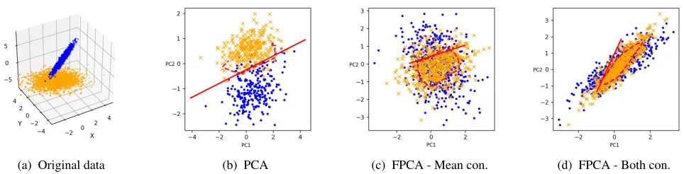
(a) Original data (b) PCA (c) FPCA - Mean con. (d) FPCA - Both con.
Figure 1: Comparison of PCA and FPCA on synthetic data. In each plot, the thick red line is the optimal linear SVM separating by color, and the dotted line is the optimal Gaussian kernel SVM.
Proof. First note that VT(Q+ϕ
I)V = VTQV +ϕIand that VT(−Q+ϕI)V = −VTQV +ϕI. Since the spec-tral norm is submultiplicative, this means kVTQVk2 ≤ kVTk2kQk2kVk2 ≤ kQk2. Soϕ ≥ kVTQVk2, and the
result follows by applying Theorem 2 toVTQV.
Recall that using the Schur complement allows represen-tation ofkV RVTk2as a positive semidefinite matrix con-straint whenRis positive semidefinite (Boyd et al. 1994). So the above corollary is useful because it means we can repre-sentkV QVTk
2using positive semidefinite matrix constraints since(Q+ϕI)and(−Q+ϕI)are positive semidefinite by construction.
5
Designing formulations for fair PCA
Consider the linear dimensionality reductionΠ(x) =VTx forV ∈ Rp×d such that VTV = I. Then for linear clas-sifier h(u, t) = 1(wTu − t ≤ 0), definition (1)sim-plifies to ∆(h) = supt|P[wTVTx ≤ t|z = +1] −
P[wTVTx ≤ t|z = −1]|. But the right-hand side is the Kolmogorov distance betweenwTVTxconditioned on z = ±1, which is upper bounded (as can be seen trivially from its definition) by the total variation distance. Conse-quently, applying Pinsker’s inequality (Massart 2007) gives
∆(h)≤q1
2KL wTVTX−
wTVTX+
,whereKL(·||·)is the Kullback-Leibler divergence,X+is the random variable [x|z= +1], andX−is the random variable[x|z=−1]. For the special caseX+∼ N(µ+,Σ+)andX−∼ N(µ−,Σ−), we have (Kullback 1997):
∆(h)≤
s
1 4
s− s+
+(m+−m−) 2
s+
+ logs+ s−
−1
. (4)
where s+ = wTVTΣ+V w, s− = wTVTΣ−V w,m+ = wTVTµ
+, andm− =wTVTµ−. The key observation here is that (4) is minimized whens+ = s− and m+ = m−, and we will use this insight to propose constraints for FPCA. IfX+ andX− are not Gaussian, the three-point property may be used to obtain a similar bound with a couple extra terms involving the divergence betweenX+ and a normal
distribution with the same mean and variance (and the analog forX−).
We first design constraints for the non-convex formulation (2) so thatmˆ+−mˆ−=wTVTfhas small magnitude, where f = ˆµ+−µˆ− = #1P Pi∈Pxi− #1N Pi∈Nxi. Note we
make the identificationP =V VTbecause of the properties ofP in (2) and sinceVTV =
I. Observe thatwTVTf is small ifVTfis small, which can be formulated as
kVTfk2=hV VT, f fTi=hP, f fTi ≤δ2, (5)
wherek · kis the`2-norm, andδis a bound on the norm. This (5) is a linear constraint onP.
We next design constraints for the non-convex formulation (2) so thatsˆ+−sˆ−=wTVT(Σ+b −Σb−)V whas small mag-nitude. Recall the identificationP =V VT because of the
properties ofPin (2) and sinceVTV =I. Next observe that wTVT(
b
Σ+−Σb−)V wis small ifVT(Σ+b −Σb−)V is small. LetQ=Σ+b −Σb−, then using Corollary 1 gives
µ+ϕ≥ kVTQVk2+ϕ
= max{kVT(Q+ϕI)Vk2,kVT(−Q+ϕI)Vk2}
= max{kV VT(Q+ϕI)V VTk2,kV VT(−Q+ϕI)V VTk2} = max{kP(Q+ϕI)Pk2,kP(−Q+ϕI)Pk2}, (6)
whereϕ ≥ kΣb+−Σb−k2, andµis a bound on the norm. Note (6) can be rewritten as SDP constraints using a standard reformulation for the spectral norm (Boyd et al. 1994).
the following SDP formulation for FPCA:
maxhXTX, Pi −µt (7a)
s.t.trace(P)≤d, IP 0 (7b)
hP, f fTi ≤δ2 (7c)
tI P M+ M+TP I
0, (7d)
tI P M− MT
−P I
0 (7e)
whereMiMiTis the Cholesky decomposition ofiQ+ϕI (i∈ {−,+}),ϕ≥ kΣ+b −Σb−k2, (7c) is called themean con-straintand denotes the use (5), and (7d) and (7e) are called thecovariance constraintsand are the SDP reformulation of (6). Our convex formulation for FPCA consists of solving (7) and then extracting thedlargest eigenvectors from the optimalP∗.
We can apply the kernel trick to (7) to develop an SDP for F-KPCA. For brevity, we only note the differences with (7): Qwould be replaced withQk =K(X, X+)K(X+, X)− K(X, X−)K(X−, X)andf withfk = #1PK(X, X+)e−
1
#NK(X, X−)e.M+andM−would then be the Cholesky decompositions of the analogous matrices, andϕwould also have to be set no less thankQkk2. K-FPCA is then the top deigenvectors of the optimal solution of the resulting SDP. Note that we may also replicate constraints (7c), (7d) & (7e) to handle multiple protected attributes. Note that they would need to be replicated further to account for interactions between protected attributes.
6
Experimental results
We use synthetic and real datasets from the UC Irvine Ma-chine Learning Repository (Lichman 2013) to demonstrate the efficacy of our SDP formulations. We also show how FPCA can be used to minimize discrimination in health in-surance rates (with respect to age). For any SVM run, tun-ing parameters were chosen ustun-ing 5-fold cross-validation, and data was normalized to have unit variance in each field. Due to constraints on space, further experimental re-sults and a overview of and comparison to the method of Calmon et al. are presented in the appendix, available at https://arxiv.org/pdf/1802.03765.pdf.
6.1
Synthetic Data
We sampled 1000 points each fromX+andX−distributed as different 3-dimensional multivariate Gaussians, and these points are shown in Figure 1a. Figure 1b displays the results of dimensionality reduction using the top two unconstrained principal components ofX: the resulting separators for linear and Gaussian kernel SVM’s are also shown. It is clear that the two sub-populations are readily distinguishable in the lower-dimensional space. Figure 1c displays the analogous information after FPCA with only the mean constraint, and Figure 1d after FPCA with both constraints. Figures 1c and 1d clearly display better mixing of the data, and the SVM’s conducted afterwards are unable to separate the sub-groups as cleanly as they can in Figure 1b; furthermore, the addition
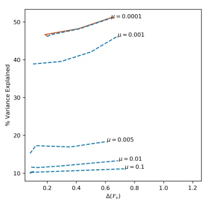
Figure 2: The sensitivity of FPCA to theδandµfor the wine quality dataset. The full red line represents FPCA with only the mean constraint, and the dotted blue lines denote FPCA with both constraints. For each curve,δ∈ {0,0.1,0.3,0.5} was considered.
of the covariance constraints (7d) incentivizes the choosing of a dimensionality reduction that better matches the skew of the entire data set.
6.2
Real data
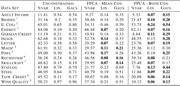
We next consider a selection of datasets from UC Irvine’s online Machine Learning Repository (Lichman 2013). For each of the datasets, one attribute was selected as a protected class, and the remaining attributes were considered part of the feature space. After splitting each dataset into separate training (70%) and testing (30%) sets, the top five principal components were then found for the training sets of each of these datasets three times: once unconstrained, once with (7) with only the mean constraints (and excluding the covariance constraints) withδ= 0, and once with (7) with both the mean and covariance constraints withδ = 0andµ = 0.01; the test data was then projected onto these vectors. All data was normalized to have unit variance in each feature, which is common practice for datasets with features of incomparable units. For each instance, we estimated∆(F)using the test set and for the families of linear SVM’sFvand Gaussian kernel SVM’s Fk. Finally, for each set of principal components V, the proportion of variance explained by the components was calculated astrace(VΣbVT))/trace(Σ)b , whereΣbis the centered sample covariance matrix of training setX. Table 1 displays all of these results averaged over 5 different training-testing splits.
Table 1:∆-fairness for both linear and Gaussian kernel SVM for PCA and FPCA. Best results for each fairness metric are bolded.
UNCONSTRAINED FPCA - MEANCON. FPCA - BOTHCON. DATASET %VAR LIN. GAUS. %VAR LIN. GAUS. %VAR LIN. GAUS.
ADULTINCOME 11.41 0.54 0.54 9.27 0.14 0.35 5.33 0.07 0.15 BIODEG1 31.16 0.2 0.35 30.46 0.14 0.29 21.45 0.10 0.28
E. COLI2 65.01 0.65 0.80 54.31 0.46 0.59 53.75 0.24 0.54 ENERGY3 84.08 0.10 0.20 66.48 0.07 0.20 62.11 0.07 0.16 GERMANCREDIT 11.19 0.21 0.31 10.91 0.14 0.33 8.84 0.11 0.29 IMAGE 62.68 0.18 0.32 52.78 0.14 0.33 48.55 0.15 0.28 LETTER 42.33 0.58 0.58 29.29 0.07 0.22 23.76 0.07 0.19 MAGIC4 61.91 0.32 0.33 29.57 0.11 0.21 25.36 0.12 0.30 PIMA5 49.00 0.30 0.37 43.98 0.17 0.26 43.26 0.18 0.25
RECIDIVISM6 56.28 0.24 0.26 46.58 0.08 0.16 39.34 0.08 0.21
SKILLCRAFT7 40.62 0.15 0.19 29.95 0.07 0.14 25.48 0.07 0.17
STATLOG 87.80 0.79 0.79 21.77 0.23 0.69 7.76 0.13 0.44 STEEL 46.05 0.64 0.71 40.79 0.19 0.51 11.86 0.09 0.22 TAIW. CREDIT8 45.52 0.11 0.17 30.07 0.08 0.16 20.08 0.06 0.14 WINEQUALITY9 50.21 0.97 0.96 37.34 0.21 0.51 10.12 0.06 0.13
in many cases, this increase in fairness comes at minimal loss in the explanatory power of the principal components. There are a few datasets for which (7d) appear superfluous. In general, gains in fairness are stronger with respect toFv; this is to be expected, asFkis a highly sophisticated set, and thus more robust to linear projections. Kernel FPCA may be a better approach to tackling this issue, but we leave this for future work. Additional experiments and a comparison to the method of Calmon et al. are shown in the appendix. We find that our method leads to more fairness on almost all datasets.
6.3
Hyperparameter sensitivity
Next, we consider the sensitivity of our results to hyperpa-rameters δ, µ, for the Wine Quality dataset. The data was split into training (70%) and testing (30%) sets, and the top three fair principle components were found using (7) with only the mean constraint for each candidateδand using (7) with both constraints for all combinations of candidateδand µ. All data was normalized to have unit variance in each independent feature. We calculated the percentage of the vari-ance explained by the resulting principle components, and we estimated the fairness level∆(Fv)for the family of linear SVM’s. This process was run 10 times for random data splits, and the averaged results are plotted in Figure 2. Here, the solid red line represents (7) with only the mean constraint. On the other hand, the dotted blue lines represent the (7) with both constraints, for the indicatedµ.
Adding the covariance constraints and further tightening µgenerally improves fairness and decreases the proportion of variance explained. However, observe that the relative sen-sitivity of fairness toδis higher than that of the variance explained, at least for this dataset. Similarly, increasingµ decreases the portion of variance explained while resulting in a less discriminatory dataset after the dimensionality re-duction. We note that increasingµpast a certain point does not provide much benefit, and so smaller values ofµare to be preferred. We found that increasingµpast 0.1 did not substantively change results further, so the largestµthat we
consider is 0.1. In general, hyperparameters may be set with cross-validation, although (4) may serve as guidance.
6.4
Fair clustering of health data
Health insurance companies are considering the use of pat-terns of physical activity as measured by activity trackers in order to adjust health insurance rates of specific individuals (Sallis, Bauman, and Pratt 1998; Paluch and Tuzovic 2017). In fact, a recent clustering analysis found that different pat-terns of physical activity are correlated with different health outcomes (Fukuoka et al. 2018). The objective of a health insurer in clustering activity data would be to find qualitative trends in an individual’s physical activity that help categorize the risks that that customer portends. That is, individuals within these activity clusters are likely to incur similar levels of medical costs, and so it would be beneficial to engineer easy-to-spot features that can help insurers bucket customers. However, health insurance rates must satisfy a number of legal fairness considerations with respect to gender, race, and age. This means that an insurance company may be found legally liable if the patterns used to adjust rates result in an unreasonably-negative impact on individuals of a specific gender, race, or age. Thus, an insurer may be interested in a feature engineering method to bucket customers while mini-mizing discrimination on protected attributes. Motivated by this, we use FPCA to perform a fair clustering of physical activity. Our goal is to find discernible qualitative trends in activity which are indicative of an individual’s activity patterns, and thus health risks, but fair with respect to age.
We use minute-level data from the the National Health and Nutrition Examination Survey (NHANES) from 2005–2006 (Centers for Desease Control and Prevention (CDC). National Center for Health Statistics (NCHS). 2018), on the intensity levels of the physical activity of about 6000 women,
mea-1 (Mansouri et al. 2013) 2 (Horton and Nakai 1996) 3 (Tsanas
and Xifara 2012) 4 (Bock et al. 2004) 5 (Smith et al. 1988) 6
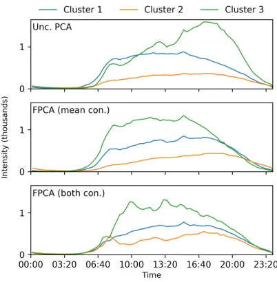
Figure 3: The mean physical activity intensities, plotted throughout a day, of the clusters generated after dimensional-ity reduction through PCA, FPCA with the mean constraint, and FPCA with both constraints. In each plot, each line repre-sents the average activity level of the members of one cluster.
sured over a week via an accelerometer. In this example, we consider age to be our protected variable, specifically whether an individual is above or below 40 years of age. We exclude weekends from our analysis, and average, over weekdays, the activity data by individual into 20-minute buckets. Thus, for each participant, we have data describing her average activity throughout an average day. We exclude individuals under 12 years of age, and those who display more than 16 hours of zero activity after averaging. The top 1% most active participants, and corrupted data, were also excluded. Finally, data points corrupted or inexact due to accelerometer mal-functioning were excluded. This preprocessing mirrors that of Fukuoka et al. and reflects practical concerns of insurers as well as the patchiness of accelerometer data.
PCA is sometimes used as a preprocessing step prior to clustering in order to expedite runtime. In this spirit, we find the top five principal components through PCA, FPCA with mean constraint, and FPCA with both constraints, withδ= 0 andµ= 0.1throughout. Then we conductk-means cluster-ing (withk= 3) on the dimensionality-reduced data for each case. Figure 3 displays the averaged physical activity patterns for the each of the clusters in each of the cases. Furthermore, Table 2 documents the proportion of each cluster comprised of examinees over 40. We note that the clusters found under an unconstrained PCA are most distinguishable after 3:00 PM, so an insurer interested in profiling an individual’s risk would largely consider their activity in the evenings. How-ever, we may observe in Table 2 that this approach results in notable age discrimination between buckets, opening the
Table 2: The proportion of each cluster that are over 40 years of age. 36.05% of all respondents are over 40. The final row displays the standard deviation of the numbers in the first three. The most fair solution would be the same age composition in all clusters, so this is a reasonable fairness metric.
UNC. MEAN BOTH
Cluster 1 43.18% 33.54% 35.61%
Cluster 2 32.94% 38.64% 36.11%
Cluster 3 8.71% 33.32% 37.28%
Std. Dev 14.87% 2.46% 1.79%
insurer to the risk of illegal price discrimination. On the hand, the second and third plots in Figure 3 and columns in Table 2 suggest that clustering customers based on their activity dur-ing the workday, between 8:00 AM and 5:00 PM, would be less prone to discrimination.
7
Conclusion
In this paper, we proposed a quantitative definition of fair-ness for dimensionality reduction, developed convex SDP formulations for fair PCA, and then demonstrated its ef-fectiveness using several datasets. Many avenues remain for future research on fair unsupervised learning. For in-stance, we believe that our formulations in this paper may have suitable modifications that can be used to develop deflation and regression approaches for fair PCA analo-gous to those for sparse PCA (d’Aspremont et al. 2007; Zou, Hastie, and Tibshirani 2006).
References
Angwin, J.; Larson, J.; Mattu, S.; and Kirchner, L. 2016. Machine bias: There’s software used across the country to predict future criminals. and it’s biased against blacks. ProP-ublica, May23.
Arora, R.; Cotter, A.; and Srebro, N. 2013. Stochastic op-timization of pca with capped msg. InAdvances in Neural Information Processing Systems, 1815–1823.
Berk, R.; Heidari, H.; Jabbari, S.; Kearns, M.; and Roth, A. 2017. Fairness in criminal justice risk assessments: The state of the art.arXiv preprint arXiv:1703.09207.
Beutel, A.; Chen, J.; Zhao, Z.; and Chi, E. H. 2017. Data deci-sions and theoretical implications when adversarially learning fair representations.arXiv preprint arXiv:1707.00075. Bock, R.; Chilingarian, A.; Gaug, M.; Hakl, F.; Hengstebeck, T.; Jiˇrina, M.; Klaschka, J.; Kotrˇc, E.; Savick`y, P.; Towers, S.; et al. 2004. Methods for multidimensional event classifica-tion: a case study using images from a cherenkov gamma-ray telescope.Nuclear Instruments and Methods in Physics Re-search Section A: Accelerators, Spectrometers, Detectors and Associated Equipment516(2):511–528.
Calders, T.; Kamiran, F.; and Pechenizkiy, M. 2009. Building classifiers with independency constraints. InData mining workshops, 2009. ICDMW’09. IEEE international confer-ence on, 13–18. IEEE.
Calmon, F.; Wei, D.; Vinzamuri, B.; Ramamurthy, K. N.; and Varshney, K. R. 2017. Optimized pre-processing for dis-crimination prevention. InAdvances in Neural Information Processing Systems, 3992–4001.
Centers for Desease Control and Prevention (CDC). National Center for Health Statistics (NCHS). 2018. National health and nutrition examination survey data.
Chierichetti, F.; Kumar, R.; Lattanzi, S.; and Vassilvitskii, S. 2017. Fair clustering through fairlets. InAdvances in Neural Information Processing Systems, 5036–5044.
Chouldechova, A. 2017. Fair prediction with disparate im-pact: A study of bias in recidivism prediction instruments. arXiv preprint arXiv:1703.00056.
Cortez, P.; Cerdeira, A.; Almeida, F.; Matos, T.; and Reis, J. 2009. Modeling wine preferences by data mining from physicochemical properties. Decision Support Systems 47(4):547–553.
d’Aspremont, A.; El Ghaoui, L.; Jordan, M.; and Lanckriet, G. 2007. A direct formulation of sparse PCA using semidefinite programming.SIAM Review49(3).
Dwork, C.; Hardt, M.; Pitassi, T.; Reingold, O.; and Zemel, R. 2012. Fairness through awareness. InProceedings of the 3rd Innovations in Theoretical Computer Science Conference, 214–226. ACM.
Feldman, M.; Friedler, S. A.; Moeller, J.; Scheidegger, C.; and Venkatasubramanian, S. 2015. Certifying and removing disparate impact. InProceedings of the 21th ACM SIGKDD International Conference on Knowledge Discovery and Data Mining, 259–268. ACM.
Fukuoka, Y.; Zhou, M.; Vittinghoff, E.; Haskell, W.; Gold-berg, K.; and Aswani, A. 2018. Objectively measured baseline physical activity patterns in women in the mped trial: Cluster analysis.JMIR Public Health and Surveillance 4(1):e10.
Hardt, M.; Price, E.; and Srebro, N. 2016. Equality of opportunity in supervised learning. InAdvances in Neural Information Processing Systems, 3315–3323.
Horton, P., and Nakai, K. 1996. A probabilistic classification system for predicting the cellular localization sites of proteins. InIsmb, volume 4, 109–115.
Kullback, S. 1997.Information theory and statistics. Courier Corporation.
Lichman, M. 2013. UCI machine learning repository. Mansouri, K.; Ringsted, T.; Ballabio, D.; Todeschini, R.; and Consonni, V. 2013. Quantitative structure–activity relation-ship models for ready biodegradability of chemicals.Journal of chemical information and modeling53(4):867–878. Massart, P. 2007. Concentration inequalities and model selection, volume 6. Springer.
Miller, C. C. 2015. Can an algorithm hire better than a human. The New York Times25.
Munoz, C.; Smith, M.; and Patil, D. 2016. Big data: A report on algorithmic systems, opportunity, and civil rights. Executive Office of the President. The White House.
Olfat, M., and Aswani, A. 2017. Spectral algorithms for computing fair support vector machines. arXiv preprint arXiv:1710.05895.
Paluch, S., and Tuzovic, S. 2017. Leveraging pushed self-tracking in the health insurance industry: How do individuals perceive smart wearables offered by insurance organization? Recht, B.; Fazel, M.; and Parrilo, P. A. 2010. Guaranteed minimum-rank solutions of linear matrix equations via nu-clear norm minimization.SIAM review52(3):471–501. Rudin, C. 2013. Predictive policing using machine learning to detect patterns of crime.Wired Magazine, August. Sallis, J.; Bauman, A.; and Pratt, M. 1998. Environmental and policy interventions to promote physical activity a.American journal of preventive medicine15(4):379–397.
Shorack, G. R., and Wellner, J. A. 2009.Empirical processes with applications to statistics, volume 59. SIAM.
Smith, J. W.; Everhart, J.; Dickson, W.; Knowler, W.; and Johannes, R. 1988. Using the adap learning algorithm to forecast the onset of diabetes mellitus. InProceedings of the Annual Symposium on Computer Application in Medical Care, 261. American Medical Informatics Association. Thompson, J. J.; Blair, M. R.; Chen, L.; and Henrey, A. J. 2013. Video game telemetry as a critical tool in the study of complex skill learning. PloS one8(9):e75129.
Tsanas, A., and Xifara, A. 2012. Accurate quantitative estimation of energy performance of residential buildings using statistical machine learning tools.Energy and Buildings 49:560–567.
Wainwright, M. 2017. High-dimensional statistics: A non-asymptotic viewpoint.
Yeh, I.-C., and Lien, C.-h. 2009. The comparisons of data mining techniques for the predictive accuracy of probabil-ity of default of credit card clients. Expert Systems with Applications36(2):2473–2480.
Zafar, M. B.; Valera, I.; Rodriguez, M. G.; and Gummadi, K. P. 2017. Fairness constraints: Mechanisms for fair classi-fication. InProceedings of the 20th International Conference on Artificial Intelligence and Statistics.
Zemel, R.; Wu, Y.; Swersky, K.; Pitassi, T.; and Dwork, C. 2013. Learning fair representations. InProceedings of the 30th International Conference on Machine Learning (ICML-13), 325–333.
Zhang, B. H.; Lemoine, B.; and Mitchell, M. 2018. Mitigat-ing unwanted biases with adversarial learnMitigat-ing.arXiv preprint arXiv:1801.07593.
Zliobaite, I. 2015. On the relation between accu-racy and fairness in binary classification. arXiv preprint arXiv:1505.05723.