Time-Domain Techniques for Computation and Reconstruction of One-Dimensional Proﬁles

(1)

SRef-ID: 1684-9973/ars/2005-3-219

Advances in

Radio Science

Time-Domain Techniques for Computation and Reconstruction of

One-Dimensional Profiles

M. Rahman and R. Marklein

Fachgebiet Theoretische Elektrotechnik, Fachbereich Elektrotechnik/Informatik, Universit¨at Kassel (UNIK), 34109 Kassel, Germany

Abstract. This paper presents a time-domain technique to compute the electromagnetic fields and to reconstruct the permittivity profile within a one-dimensional medium of fi-nite length. The medium is characterized by a permittivity as well as conductivity profile which vary only with depth. The discussed scattering problem is thus one-dimensional. The modeling tool is divided into two different schemes which are named as the forward solver and the inverse solver. The task of the forward solver is to compute the internal fields of the specimen which is performed by Greens function ap-proach. When a known electromagnetic wave is incident nor-mally on the media, the resulting electromagnetic field within the media can be calculated by constructing a Greens oper-ator. This operator maps the incident field on either side of the medium to the field at an arbitrary observation point. It is nothing but a matrix of integral operators with kernels satis-fying known partial differential equations. The reflection and transmission behavior of the medium is also determined from the boundary values of the Green’s operator. The inverse solver is responsible for solving an inverse scattering prob-lem by reconstructing the permittivity profile of the medium. Though it is possible to use several algorithms to solve this problem, the invariant embedding method, also known as the layer-stripping method, has been implemented here due to the advantage that it requires a finite time trace of reflection data. Here only one round trip of reflection data is used, where one round trip is defined by the time required by the pulse to propagate through the medium and back again. The inversion process begins by retrieving the reflection kernel from the reflected wave data by simply using a deconvolu-tion technique. The rest of the task can easily be performed by applying a numerical approach to determine different pro-file parameters. Both the solvers have been found to have the ability to deal with different types of slabs and incident elec-tromagnetic pulses. Slabs having continuous and discontin-uous relative permittivity have already been tested success-fully. The tested electromagnetic pulses are a Dirac, Gaus-sian and sinusoidal pulse. Due to sampling, the resolution of the system also plays a significant role in obtaining better outputs from this scheme.

Correspondence to: R. Marklein ([email protected])

1 Introduction

Recently, 1-D profiling has become a point of high inter-est, for instance in geophysics and Non-Destructive Testing (NDT), not only due to the ease to solve the problems ana-lytically but also due to high accuracy level. They have large importance in Time Domain Reflectometry (TDR) such as moisture meter and material analysis (Connor and Dowding, 1999; Schlaeger, 2002). The forward solver of such schemes works on a known slab and determines the electromagnetic field. On the other hand, the inverse solver takes the reflec-tion data from the slab as an input and determines the prop-erties of the unknown slab. The known methods to solve the forward problem are

– Finite-Difference Time-Domain (FDTD) method (Taflove and Hagness, 2000)

– Finite Integration Technique (FIT) (Marklein, 2002)

– Green’s function approach (Krueger and Ochs Jr., 1989).

The Green’s function approach has some advantages over the other methods. Firstly, in this method the wave equation needs not to be solved for each incident wave form. Sec-ondly, wave field throughout the entire medium does not have to be computed. For these advantages, this method has been implemented in the forward solver. The inverse problem can be solved by

– invariant embedding (layer stripping) (Corones et al., 1983)

– downward continuation (Green’s function approach) (Kristensson and Krueger, 1986, 1987).

(2)

220 M. Rahman and R. Marklein: Computation and Reconstruction of One-Dimensional Profiles 2 M. Rahman and R. Marklein: Computation and Reconstruction of One-Dimensional Profiles 2 Statement of the problem

The geometry of the problem is shown in Fig. 1. An inho-mogeneous slab occupies the region0≤z≤L. The permit-tivity and conducpermit-tivity profiles are functions of depthzonly. A homogeneous, lossless medium is situated on either side

Inhomogeneous

Homogeneous Homogeneous

ε

1

1,σ0 ε2,σ0

ε(z) σ(z)

0 L z

Fig. 1. Geometry of the inhomogeneous slab.

of the slab. The electric field strengthE(z, t)within the slab can be expressed by

∂2

∂z2E(z, t)− 1 c2₍_z₎

∂2

∂t2E(z, t)−b(z)

∂

∂tE(z, t) = 0, (1) where

c−₂

(z) =ε(z)µ0 , b(z) =σ(z)µ0. (2)

Hereµ0,σ(z)andε(z)represent the permeability of

vac-uum, conductivity and permittivity respectively. The phase velocityc(z)is assumed to be continuous at the boundary, which means

c(z) =c(0+), z≤0 ; c(z) =c(L−), z≥L . (3) 2.1 Normalization

In order to facilitate the numerical computations a conversion to travel time coordinates is made. These coordinates are defined as

l=

Z L 0

1

c(z)dz , s(t) =t/l (4) x=x(z) =

Z z z0=0

1 lc(z0₎dz

0

, u(x, s) =E(z, t), (5) wherexis normalized distance andsis normalized time. The slab occupies the region0≤x≤1and a round trip time is described by0< s <2which is equivalent to2l. In fact,l represents the time taken by the wave front to travel through the slab once. So the wave equation will be transformed into

∂2

∂x2u(x, s)−

∂2

∂s2u(x, s) +A(x)

∂ ∂xu(x, s)

+B(x) ∂

∂su(x, s) = 0, (6) where

A(x) =− d

dx lnc[z(x)] (7)

B(x) =−l b[z(x)]c2[z(x)]. (8)

-Fig. 2. Wave splitting.

2.2 Wave splitting

The wave travelling in the non-homogeneous slab can be splitted into left- and right-going parts. In Fig. 2, u+₍_{x, s}₎

is the right going wave andu−

(x, s)is the left going wave. For all times, the initial and boundary conditions are

u+(x,0) =u−

(x,0) = 0 ; 0< x <1 (9) u+(0, s) =f(s) , u−

(1, s) = 0 ; s >0. (10) An incident wave is impinged only from the left side which is denoted byf(s).

3 Forward solver: introduction to the Green’s kernel The known parameters are incident pulse, slab lengthL,εr

andσ profile. The goal is to determine the internal fields. A matrix operator[G_](_x₎_{can be defined to map the incident} wavesu+₍₀_{, s}₎_,_u−

(1, s)to internal fieldsu+₍_{x, s}₎_,_u− (x, s)

u+₍_{x, s}₎

u− (x, s)

=

G11(x)G12(x)

G21(x)G22(x)

| {z }

=[G](x)

u+₍₀_{, s}₎

u− (1, s)

. (11)

Considering an incident wave only from left side, we find u+₍_{x, s}_{) =}_G

11(x)∗f(s)

u−

(x, s) =G21(x)∗f(s)

; as u+₍₀_{, s}_{) =}_f₍_s₎_, ₍₁₂₎

where ”∗” denotes convolution. G11,G21are related to the

forward and backward travelling wave, respectively, when the incident wave is applied from the left side of the slab. G12,G22are not considered here as they are only applicable

for an incident wave coming from the right side of the slab. Now by applying Duhamel’s integral,

u+₍_{x, s}_{) =}_t+₍₀_{, x}₎_{_f₍_s₋_x₎

+

Z s−x 0

f(s0

)G11(x, s−s

0 )ds0

(13) u−

(x, s) = 1 t−₍₀_{, x}₎

Z s−x 0

f(s0

)G21(x, s−s

0 )ds0

, (14) where

t±(x1, x2) = exp

±1 2

Z x2 x1

[A(x0]∓B(x0)]dx0

. (15) 3.1 Equations of the Green’s kernel

The fieldsu+₍_{x, s}₎_and_u−

(x, s)satisfy the following equa-tion

∂ ∂x

u+₍_{x, s}₎

u− (x, s)

=

α(x)β(x) γ(x)δ(x)

u+₍_{x, s}₎

u− (x, s)

, (16)

2 Statement of the problem

The geometry of the problem is shown in Fig. 1. An inhomo-geneous slab occupies the region 0≤z≤L. The permittivity and conductivity profiles are functions of depthzonly.

A homogeneous, lossless medium is situated on either side of the slab. The electric field strengthE(z, t )within the slab can be expressed by

∂2

∂z2E(z, t )−

1

c2_(z)

∂2

∂t2E(z, t )−b(z)

∂

∂tE(z, t )=0, (1)

where

c−2(z)=ε(z) µ0 , b(z)=σ (z) µ0. (2)

Hereµ0, σ (z)and ε(z)represent the permeability of

c(z)=c(0+), z≤0 ; c(z)=c(L−), z≥L . (3) 2.1 Normalization

l= Z L

0

1

c(z)dz , s(t )=t / l (4)

x=x(z)= Z z

z0₌₀

1

lc(z0₎dz 0

, u(x, s)=E(z, t ) , (5) wherexis normalized distance andsis normalized time. The slab occupies the region 0≤x≤1 and a round trip time is de-scribed by 0<s<2 which is equivalent to 2l. In fact,l rep-resents the time taken by the wave front to travel through the slab once. So the wave equation will be transformed into

∂2

∂x2u(x, s)−

∂2

∂s2u(x, s)+A(x)

∂ ∂xu(x, s)

+B(x) ∂

∂su(x, s)=0, (6)

where

A(x)= − d

dx lnc[z(x)] (7)

B(x)= −l b[z(x)]c2[z(x)]. (8)

2 M. Rahman and R. Marklein: Computation and Reconstruction of One-Dimensional Profiles 2 Statement of the problem

The geometry of the problem is shown in Fig. 1. An inho-mogeneous slab occupies the region0≤z≤L. The permit-tivity and conducpermit-tivity profiles are functions of depthzonly. A homogeneous, lossless medium is situated on either side

Inhomogeneous

Homogeneous Homogeneous

ε

1

1,σ0 ε2,σ0

ε(z) σ(z)

0 L z

of the slab. The electric field strengthE(z, t)within the slab can be expressed by

∂2

∂z2E(z, t)− 1 c2₍_z₎

∂2

∂t2E(z, t)−b(z)

∂

∂tE(z, t) = 0, (1) where

c−2(z) =ε(z)µ0 , b(z) =σ(z)µ0. (2)

Hereµ0, σ(z)andε(z)represent the permeability of

c(z) =c(0+), z≤0 ; c(z) =c(L−), z≥L . (3) 2.1 Normalization

l=

Z L 0

1

c(z)dz , s(t) =t/l (4) x=x(z) =

Z z z0=0

1 lc(z0

)dz 0

, u(x, s) =E(z, t), (5) wherexis normalized distance andsis normalized time. The slab occupies the region0≤x≤1and a round trip time is described by0< s <2which is equivalent to2l. In fact,l represents the time taken by the wave front to travel through the slab once. So the wave equation will be transformed into

∂2

∂x2u(x, s)−

∂2

∂s2u(x, s) +A(x)

∂ ∂xu(x, s)

+B(x) ∂

∂su(x, s) = 0, (6) where

A(x) =− d

dx lnc[z(x)] (7)

B(x) =−l b[z(x)]c2[z(x)]. (8)

-Fig. 2. Wave splitting.

2.2 Wave splitting

The wave travelling in the non-homogeneous slab can be splitted into left- and right-going parts. In Fig. 2, u+₍_{x, s}₎

is the right going wave andu−

(x, s)is the left going wave. For all times, the initial and boundary conditions are

u+(x,0) =u−(x,0) = 0 ; 0< x <1 (9) u+₍₀_{, s}_{) =}_f₍_s₎ _{, u}−

(1, s) = 0 ; s >0. (10) An incident wave is impinged only from the left side which is denoted byf(s).

andσ profile. The goal is to determine the internal fields. A matrix operator[G_](_x₎_{can be defined to map the incident} wavesu+₍₀_{, s}₎_,_u−

(1, s)to internal fieldsu+₍_{x, s}₎_,_u− (x, s)

u+₍_{x, s}₎

u− (x, s)

=

G11(x)G12(x)

G21(x)G22(x)

| {z }

=[G](x)

u+₍₀_{, s}₎

u− (1, s)

. (11)

Considering an incident wave only from left side, we find u+₍_{x, s}_{) =}_G

11(x)∗f(s)

u−

(x, s) =G21(x)∗f(s)

; as u+₍₀_{, s}_{) =}_f₍_s₎_, ₍₁₂₎

where ”∗” denotes convolution. G11,G21are related to the

forward and backward travelling wave, respectively, when the incident wave is applied from the left side of the slab. G12,G22are not considered here as they are only applicable

u+(x, s) =t+(0, x){f(s−x)

+

Z s−x 0

f(s0

)G11(x, s−s0)ds0

(13) u−(x, s) = 1

t−₍₀_{, x}₎

Z s−x 0

f(s0)G21(x, s−s

0

)ds0, (14) where

t±

(x1, x2) = exp

±1 2

Z x2 x1

[A(x0

]∓B(x0 )]dx0

. (15) 3.1 Equations of the Green’s kernel

The fieldsu+₍_{x, s}₎_and_u−

(x, s)satisfy the following equa-tion

∂ ∂x

u+₍_{x, s}₎

u− (x, s)

=

u+₍_{x, s}₎

u− (x, s)

, (16)

Fig. 2. Wave splitting.

2.2 Wave splitting

The wave travelling in the non-homogeneous slab can be splitted into left- and right-going parts. In Fig. 2,u+(x, s)

is the right going wave andu−(x, s)is the left going wave. For all times, the initial and boundary conditions are

u+(x,0)=u−(x,0)=0 ; 0< x <1 (9)

u+(0, s)=f (s) , u−(1, s)=0 ; s >0. (10) An incident wave is impinged only from the left side which is denoted byf (s).

andσ profile. The goal is to determine the internal fields. A matrix operator[G](x)can be defined to map the incident wavesu+(0, s),u−(1, s)to internal fieldsu+(x, s),u−(x, s)

u+(x, s) u−(x, s)

=

G11(x) G12(x)

G21(x) G22(x)

| {z }

=[G](x)

u+(0, s) u−(1, s)

. (11)

Considering an incident wave only from left side, we find

u+(x, s)=G11(x)∗f (s)

u−(x, s)=G21(x)∗f (s)

; as u+(0, s)=f (s) ,(12)

where ”∗” denotes convolution. G11,G21 are related to the

forward and backward travelling wave, respectively, when the incident wave is applied from the left side of the slab.

G12,G22are not considered here as they are only applicable

u+(x, s)=t+(0, x){f (s−x)

+ Z s−x

0

f (s0) G11(x, s−s0)ds0

(13)

u−(x, s)= 1

t−₍₀_{, x)}

Z s−x

0

f (s0) G21(x, s−s0)ds0, (14)

where

t±(x1, x2)=exp

±1

2 Z x2

x1

[A(x0] ∓B(x0)]dx0

(3)

Fig. 3. Conditions of the Green’s kernel.

whereα(x),β(x),γ(x), andδ(x)are the functions ofA(x), B(x)and incorporate time derivative_∂s∂. From Eqs. (11) and (10), it can be summarized that

∂

∂x[G](x) =

α(x)β(x) γ(x) δ(x)

G11(x)G12(x)

G21(x)G22(x)

. (17)

Again using Eq. (7), it can be shown that ∂

∂x[G11(x)f] (s) =α(x) [G11(x)f] (s)

+β(x) [G21(x)f] (s). (18)

Substituting[G11(x)f](s)by the right side of the Eq. (13), a

simple expression ofG11can be obtained, as follows

∂

∂xG11(x, s) + ∂

∂sG11(x, s) = 1

2[A(x) +B(x)] exp

−

Z x 0

B(x0 )dx0

G21(x, s). (19)

Similarly using Eq. (14),G21can be defined as

∂

∂xG21(x, s) + ∂

∂sG21(x, s) = 1

2[A(x)−B(x)] exp

Z x 0

B(x0)dx0

G11(x, s). (20)

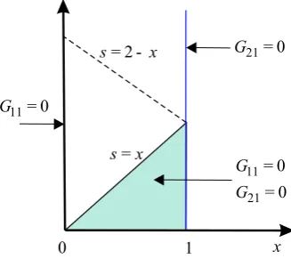
3.2 Initial, boundary, and jump conditions

G11is continuous everywhere except ons=x(see Fig. 3).

On this line the kernels can be expressed as G11(x, x+) =−

1 8

Z x 0

[A2(x0

)−B2(x0 )]dx0

(21) G21(x, x+) =−1

4[A(x)−B(x)] exp

Z x 0

B(x0 )dx0

. (22) Again on the lines= 2−x,

G21(x,(2−x)+)−G21(x,(2−x)−)

= 1

4[A(1)−B(1)] exp

Z 1 0

B(x0)dx0

. (23)

The initial and boundary conditions can be defined as G11(x, s) =G21(x, s) = 0 ; s < x (24)

G11(0, s) =G21(1, s) = 0 ; s >0. (25)

Computational Molecule

1,

i- j i-1,j+1 ,

i j s=x

2 s= - x

0 j=

j=N-i

Fig. 4. Computational molecule and variable transformation.

3.3 Numerical implementation of the forward solver The Green’s kernels explained by Eqs. (19) and (20) can also be implemented numerically. By fixing a constant∆, the first equation can be integrated from(x−∆, s−∆)to(x, s)along the characteristicss−x =const. and the second one from (x, s)to(x+∆, s−∆)along the characteristicss+x=const. with approximating the right-hand side by trapezoidal rule. So the equations will become

G11(x, s)−G11(x−∆, s−∆) =a(x)G21(x, s)

+a(x−∆)G21(x−∆, s−∆) +O(∆3) (26)

G21(x+ ∆, s−∆)−G21(x, s) =b(x)G11(x, s)

+b(x+ ∆)G11(x+ ∆, s−∆) +O(∆3), (27)

where a(x) = 1

4∆[A(x) +B(x)] exp

−

Z x x0=0

B(x0)dx0

(28) b(x) = 1

4∆[A(x)−B(x)] exp

Z x x0₌₀

B(x0)dx0

. (29) Let us now introduce a grid of points as shown in Fig. 4: (xi, si+2j) = (i∆,(i+ 2j)∆),i = 0, . . . , N; j = 0, . . . HereNrepresents the total number of grid points. Consider-ing∆ = 1/N, it can be stated that

Gi,j₁₁ =G11(i∆,(i+ 2j)∆) , ai=a(i∆) (30)

Gi,j21 =G21(i∆,(i+ 2j)∆) , bi=b(i∆). (31)

Using these approximations, Eqs. (26) and (27) can be rewritten as

Gi,j₁₁ =dih_Gi−1,j

11 +a

i−1_Gi−1,j

21 −a

i_bi+1_Gi+1,j−1 11 +aiGi21+1,j−1

i

(32) Gi,j21 =di

h

−bi_Gi−1,j

11 −ai

−1_bi_Gi−1,j

21 −bi+1G i+1,j−1 11 +Gi21+1,j−1

i

, (33)

where

di_{= [1 +}_ai_bi_]−1₌

1 + 1 16∆

2₍_A2₍_i_∆)₋_B2₍_i_∆))

−1

. (34) andi = 1,2, . . . , N−1;j = 1,2, . . .The initial condition represented by s = x, i.e., j = 0, can be determined by Eqs. (21) and (22). The boundary conditions are

G011,j = 0, G N,j

21 = 0; j= 0,1,2, ... (35) Fig. 3. Conditions of the Green’s kernel.

3.1 Equations of the Green’s kernel

The fieldsu+(x, s)andu−(x, s)satisfy the following equa-tion

∂ ∂x

u+(x, s) u−(x, s)

=

α(x) β(x) γ (x) δ(x)

u+(x, s) u−(x, s)

, (16)

whereα(x),β(x),γ (x), andδ(x)are the functions ofA(x),

B(x)and incorporate time derivative_∂s∂. From Eqs. (11) and (10), it can be summarized that

∂

∂x[G](x)=

α(x) β(x) γ (x) δ(x)

G11(x) G12(x)

G21(x) G22(x)

. (17)

Again using Eq. (7), it can be shown that

∂

∂x[G11(x) f](s)=α(x)[G11(x) f](s)

+β(x)[G21(x) f](s) . (18)

Substituting[G11(x) f](s)by the right side of the Eq. (13),

a simple expression ofG11can be obtained, as follows

∂

∂xG11(x, s)+ ∂

∂sG11(x, s)

=1

2[A(x)+B(x)]exp

− Z x

0

B(x0)dx0

G21(x, s) . (19)

∂

∂xG21(x, s)+ ∂

∂sG21(x, s)

=1

2[A(x)−B(x)]exp

Z x

0

B(x0)dx0

G11(x, s) . (20)

G11 is continuous everywhere except ons=x (see Fig. 3).

On this line the kernels can be expressed as

G11(x, x+)= −

1 8

Z x

0

[A2(x0)−B2(x0)]dx0 (21)

G21(x, x+)= −

1

4[A(x)−B(x)]exp

Z x

0

B(x0)dx0

.(22)

Fig. 3. Conditions of the Green’s kernel.

whereα(x),β(x),γ(x), andδ(x)are the functions ofA(x), B(x)and incorporate time derivative_∂s∂. From Eqs. (11) and (10), it can be summarized that

∂

∂x[G](x) =

G11(x)G12(x)

G21(x)G22(x)

. (17)

Again using Eq. (7), it can be shown that ∂

∂x[G11(x)f] (s) =α(x) [G11(x)f] (s)

+β(x) [G21(x)f] (s). (18)

Substituting[G11(x)f](s)by the right side of the Eq. (13), a

simple expression ofG11can be obtained, as follows

∂

∂xG11(x, s) + ∂

∂sG11(x, s) = 1

2[A(x) +B(x)] exp

−

Z x 0

B(x0)dx0

G21(x, s).(19)

∂

∂xG21(x, s) + ∂

∂sG21(x, s) = 1

2[A(x)−B(x)] exp

Z x 0

B(x0 )dx0

G11(x, s). (20)

G11is continuous everywhere except ons=x(see Fig. 3).

On this line the kernels can be expressed as G11(x, x+) =−1

8

Z x 0

[A2(x0)−B2(x0)]dx0 (21) G21(x, x+) =−1

4[A(x)−B(x)] exp

Z x 0

B(x0)dx0

. (22) Again on the lines= 2−x,

G21(x,(2−x)+)−G21(x,(2−x)−)

= 1

4[A(1)−B(1)] exp

Z 1 0

B(x0 )dx0

. (23)

The initial and boundary conditions can be defined as G11(x, s) =G21(x, s) = 0 ; s < x (24)

G11(0, s) =G21(1, s) = 0 ; s >0. (25)

Computational Molecule

1,

i- j i-1,j+1 ,

i j s=x

2

s= - x

0

j=

j=N-i

Fig. 4. Computational molecule and variable transformation.

3.3 Numerical implementation of the forward solver The Green’s kernels explained by Eqs. (19) and (20) can also be implemented numerically. By fixing a constant∆, the first equation can be integrated from(x−∆, s−∆)to(x, s)along the characteristicss−x =const. and the second one from (x, s)to(x+∆, s−∆)along the characteristicss+x=const. with approximating the right-hand side by trapezoidal rule. So the equations will become

G11(x, s)−G11(x−∆, s−∆) =a(x)G21(x, s)

+a(x−∆)G21(x−∆, s−∆) +O(∆3) (26)

G21(x+ ∆, s−∆)−G21(x, s) =b(x)G11(x, s)

+b(x+ ∆)G11(x+ ∆, s−∆) +O(∆3), (27)

where a(x) =1

4∆[A(x) +B(x)] exp

−

Z x x0₌₀

B(x0)dx0

(28) b(x) =1

4∆[A(x)−B(x)] exp

Z x x0=0

B(x0 )dx0

. (29) Let us now introduce a grid of points as shown in Fig. 4: (xi, si+2j) = (i∆,(i+ 2j)∆),i = 0, . . . , N; j = 0, . . . HereNrepresents the total number of grid points. Consider-ing∆ = 1/N, it can be stated that

Gi,j11 =G11(i∆,(i+ 2j)∆) , ai=a(i∆) (30)

Gi,j21 =G21(i∆,(i+ 2j)∆) , bi=b(i∆). (31)

Gi,j₁₁ =dih_Gi−1,j

11 +ai

−1_Gi−1,j

21 −aibi+1G i+1,j−1 11 +ai_Gi+1,j−1

21

i

(32) Gi,j21 =di

h

−biGi11−1,j−ai

−1_bi_Gi−1,j

21 −bi+1G i+1,j−1 11

+Gi₂₁+1,j−1i, (33) where

di_{= [1 +}_ai_bi_]−1₌_{1 +} 1 16∆

2₍_A2₍_i_∆)₋_B2₍_i_∆))

−1

. (34) andi = 1,2, . . . , N −1;j = 1,2, . . .The initial condition represented bys = x, i.e., j = 0, can be determined by Eqs. (21) and (22). The boundary conditions are

G011,j = 0, G N,j

21 = 0; j= 0,1,2, ... (35) Fig. 4. Computational molecule and variable transformation.

Again on the lines=2−x,

G21(x, (2−x)+)−G21(x, (2−x)−)

= 1

4[A(1)−B(1)]exp (

Z 1

0

B(x0)dx0

)

. (23)

The initial and boundary conditions can be defined as

G11(x, s)=G21(x, s)=0 ; s < x (24)

G11(0, s)=G21(1, s)=0 ; s >0. (25)

3.3 Numerical implementation of the forward solver The Green’s kernels explained by Eqs. (19) and (20) can also be implemented numerically. By fixing a constant1, the first equation can be integrated from(x−1, s−1)to(x, s)along the characteristics s−x=const. and the second one from

(x, s)to(x+1, s−1)along the characteristicss+x=const. with approximating the right-hand side by trapezoidal rule. So the equations will become

G11(x, s)−G11(x−1, s−1)=a(x)G21(x, s)

+a(x−1)G21(x−1, s−1)+O(13) (26)

G21(x+1, s−1)−G21(x, s)=b(x)G11(x, s)

+b(x+1)G11(x+1, s−1)+O(13) , (27)

where

a(x)= 1

41[A(x)+B(x)]exp

− Z x

x0₌₀

B(x0)dx0

(28)

b(x)= 1

41[A(x)−B(x)]exp

Z x

x0₌₀

B(x0)dx0

. (29)

Let us now introduce a grid of points as shown in Fig. 4:

(xi, si+2j)=(i 1, (i+2j )1),i=0, . . . , N;j=0, . . .HereN represents the total number of grid points. Considering

1=1/N, it can be stated that

Gi,j₁₁ =G11(i 1, (i+2j )1) , ai =a(i 1) (30)

Gi,j₂₁ =G21(i 1, (i+2j )1) , bi =b(i 1) . (31)

Gi,j₁₁ =dihGi−₁₁1,j+ai−1G₂₁i−1,j−aibi+1Gi₁₁+1,j−1

+aiGi+₂₁1,j−1i (32)

Gi,j₂₁ =dih−biGi−₁₁1,j−ai−1biGi−₂₁1,j−bi+1Gi₁₁+1,j−1

+Gi₂₁+1,j−1

i

(4)

222 M. Rahman and R. Marklein: Computation and Reconstruction of One-Dimensional Profiles 4 M. Rahman and R. Marklein: Computation and Reconstruction of One-Dimensional Profiles To incorporate the discontinuity ofG21on the lines= 2−x,

i.e. j = N−i,Gi,N21 −ibelow the line can be computed by

Eq. (33). Above this line,(Gi,N21 −i)+can be determined by

Gi,N21 −i

+

=Gi,N21 −i

−

+1

4[A(1)−B(1)] exp

Z 1 0

B(x)dx

. (36)

This value is used in place ofGi,N21 −idetermined by Eq. (33)

while computingGi,N11 −i+1andG i,N−i+1

21 .

3.4 Software implementation of the forward solver This scheme has already been tested to simulate sinusoidal, square and multiple Gaussian shapedεrprofiles. Considered

electromagnetic pulses are: Dirac pulse, Gaussian pulse, five pulses of sinusoidal wave, raised cosine and step function. The results have been tested in both lossless and lossy con-dition. A multiple Gaussian shaped slab with incident Gaus-sian pulse has been simulated here (see Figs. 5 and 6).

0 0.002 0.004 0.006 0.008 0.01 1

2 3

z in m −>

ε r

0 0.002 0.004 0.006 0.008 0.01 0

0.5 1

z in m −>

σ

0 0.4 0.8 1.2 1.6 2

0 2

s −>

Volt

Fig. 5. Top:εrprofile; Middle:σprofile; Bottom: incident pulse. Slab lengthL= 1cm, number of cells in bothz_andx_{direction is} 512, grid size∆ = 1.95_×10−5_{m and}_∆t= 85ps.

4 Inverse solver: layer stripping

The necessary data to start inversion are the length of the slab L, incident pulse (as reference), relative permittivityε1of the

first medium (surrounding medium) and measured reflection data. The desired goal is to determine the unknown relative permittivityεr profile of the slab. In the inversion scheme,

the slab is assumed to be lossless, so the conductivityσ be-comes zero. From the wave splitting phenomenon, it can be shown that

E(z, t) =E+(z, t) +E−

(z, t). (37)

Fig. 6. Left: Total fieldE_{total; Middle: Incident field}E+_{; Right:}

Reflected fieldE−_.

The backward travelling wave E−

(z, t) can be associated with reflection kernelR+₍_{z, t}₎_{in the following way}

E−(z, t) =E+(z, t)∗R+(z, t). (38)

Layer

0 1 2 3

-Fig. 7. Wave splitting and layer approach.

The reflection data obtained from measurement can be men-tioned asE−

(0, t)at the first layer (see Fig. 7). To find the reflection kernel R+₍₀_{, t}₎_{at this layer, we have to perform}

deconvolution. As a result R+₍₀_{, t}_{) = decon}_{_E−

(0, t), f(t)}asf(t) =E+₍₀_{, t}₎_.(39)

4.1 Input data processing

As deconvolution is much easier to perform in frequency do-main, the time domain parameters f(t)and E−

(0, t) will be transformed into frequency domain parametersF(ω)and E−₍_ω₎_{at first by using Fast Fourier Transform (FFT). Then} in frequency domain it can be written as

E−

(ω) =R+(ω)F(ω) ⇒ R+(ω) =E−

(ω)/F(ω).(40) The obtained data should be filtered in order to avoid zeros which might occur at the deconvolution step. A Hanning window is used in this scheme as a filter. At the end,R+₍_ω₎

is converted intoR+₍₀_{, t}₎_{by Inverse Fast Fourier Transform}

(IFFT). Then the reflection data from the first layer will be used to initiate the reconstruction process.

Fig. 5. Top:εrprofile; Middle:σ profile; Bottom: incident pulse.

Slab lengthL=1 cm, number of cells in bothzandxdirection is 512, grid size1=1.95×10−5m and1t=85 ps.

where

di = [1+aibi]−1=

1+ 1 161

2_(A2_{(i 1)}₋_B2_{(i 1))}

−1

.

(34) andi=1,2, . . . , N−1;j=1,2, . . .The initial condition rep-resented bys=x, i.e.,j=0, can be determined by Eqs. (21) and (22). The boundary conditions are

G0₁₁,j =0, GN ,j₂₁ =0; j =0,1,2, ... (35) To incorporate the discontinuity ofG21 on the lines=2−x,

i.e. j=N−i, Gi,N−i₂₁ below the line can be computed by Eq. (33). Above this line,(Gi,N−i₂₁ )+can be determined by

Gi,N−i₂₁

+

=Gi,N−i₂₁

−

+1

4[A(1)−B(1)] exp (

Z 1

0

B(x)dx

)

. (36)

This value is used in place ofGi,N−i₂₁ determined by Eq. (33) while computingGi,N−i+₁₁ 1andGi,N−i+₂₁ 1.

The necessary data to start inversion are the length of the slab

L, incident pulse (as reference), relative permittivityε1of the

4 M. Rahman and R. Marklein: Computation and Reconstruction of One-Dimensional Profiles To incorporate the discontinuity ofG21on the lines= 2−x,

i.e. j =N −i,Gi,N21 −i below the line can be computed by

Eq. (33). Above this line,(Gi,N₂₁ −i)+_{can be determined by}

Gi,N21 −i

+

=Gi,N21 −i

−

+1

4[A(1)−B(1)] exp

Z 1 0

B(x)dx

. (36)

This value is used in place ofGi,N21 −idetermined by Eq. (33)

while computingGi,N11 −i+1andG i,N−i+1

21 .

0 0.002 0.004 0.006 0.008 0.01 1

2 3

z in m −>

ε r

0 0.002 0.004 0.006 0.008 0.01 0

0.5 1

z in m −>

σ

0 0.4 0.8 1.2 1.6 2

0 2

s −>

Volt

Fig. 5. Top:εrprofile; Middle: σprofile; Bottom: incident pulse. Slab lengthL= 1cm, number of cells in bothz_andx_{direction is} 512_{, grid size}∆ = 1.95_×10−5_{m and}∆t= 85_ps.

first medium (surrounding medium) and measured reflection data. The desired goal is to determine the unknown relative permittivityεr profile of the slab. In the inversion scheme,

E(z, t) =E+₍_{z, t}_{) +}_E−

(z, t). (37)

Fig. 6. Left: Total fieldE_{total; Middle: Incident field}E+_{; Right:}

Reflected fieldE−_.

The backward travelling wave E−₍_{z, t}₎ _{can be associated} with reflection kernelR+₍_{z, t}₎_{in the following way}

E−

(z, t) =E+(z, t)∗R+(z, t). (38)

Layer

0 1 2 3

(0, t)at the first layer (see Fig. 7). To find the reflection kernelR+₍₀_{, t}₎_{at this layer, we have to perform}

deconvolution. As a result

R+(0, t) = decon{E−(0, t), f(t)}asf(t) =E+(0, t).(39)

As deconvolution is much easier to perform in frequency do-main, the time domain parameters f(t) andE−

(0, t)will be transformed into frequency domain parametersF(ω)and E−₍_ω₎_{at first by using Fast Fourier Transform (FFT). Then} in frequency domain it can be written as

E−

(ω) =R+(ω)F(ω) ⇒ R+(ω) =E−

Fig. 6. Left: Total fieldEtotal; Middle: Incident fieldE+; Right:

Reflected fieldE−.

4 M. Rahman and R. Marklein: Computation and Reconstruction of One-Dimensional Profiles To incorporate the discontinuity ofG21on the lines= 2−x,

i.e. j = N−i,Gi,N₂₁ −ibelow the line can be computed by Eq. (33). Above this line,(Gi,N₂₁−i)+_{can be determined by}

Gi,N₂₁ −i+=Gi,N₂₁ −i −

+1

4[A(1)−B(1)] exp

Z 1 0

B(x)dx

. (36)

This value is used in place ofGi,N₂₁ −idetermined by Eq. (33) while computingGi,N₁₁−i+1andGi,N₂₁ −i+1.

0 0.002 0.004 0.006 0.008 0.01 1

2 3

z in m −>

ε r

0 0.002 0.004 0.006 0.008 0.01 0

0.5 1

z in m −>

σ

0 0.4 0.8 1.2 1.6 2

0 2

s −>

Volt

Fig. 5. Top:εrprofile; Middle:σprofile; Bottom: incident pulse. Slab lengthL= 1cm, number of cells in bothz_andx_{direction is} 512, grid size∆ = 1.95_×10−5_{m and}_∆_t_{= 85}_ps.

first medium (surrounding medium) and measured reflection data. The desired goal is to determine the unknown relative permittivityεrprofile of the slab. In the inversion scheme,

E(z, t) =E+(z, t) +E−(z, t). (37)

Fig. 6. Left: Total fieldE_{total; Middle: Incident field}E+ ; Right: Reflected fieldE−_.

The backward travelling wave E−

(z, t) can be associated with reflection kernelR+₍_{z, t}₎_{in the following way}

E−

(z, t) =E+(z, t)∗R+(z, t). (38)

Layer

0 1 2 3

(0, t)at the first layer (see Fig. 7). To find the reflection kernelR+₍₀_{, t}₎_{at this layer, we have to perform}

deconvolution. As a result

R+(0, t) = decon{E−(0, t), f(t)}asf(t) =E+(0, t).(39)

As deconvolution is much easier to perform in frequency do-main, the time domain parameters f(t)and E−

(0, t)will be transformed into frequency domain parametersF(ω)and E−

(ω)at first by using Fast Fourier Transform (FFT). Then in frequency domain it can be written as

E−

(ω) =R+(ω)F(ω) ⇒ R+(ω) =E−

Fig. 7. Wave splitting and layer approach.

first medium (surrounding medium) and measured reflection data. The desired goal is to determine the unknown relative permittivityεrprofile of the slab. In the inversion scheme, the

slab is assumed to be lossless, so the conductivityσbecomes zero. From the wave splitting phenomenon, it can be shown that

E(z, t )=E+(z, t )+E−(z, t ) . (37)

The backward travelling wave E−(z, t ) can be associated with reflection kernelR+(z, t )in the following way

E−(z, t )=E+(z, t )∗R+(z, t ) . (38)

The reflection data obtained from measurement can be men-tioned asE−(0, t )at the first layer (see Fig. 7). To find the reflection kernelR+(0, t ) at this layer, we have to perform deconvolution. As a result

R+(0, t )=decon{E−(0, t ), f (t )}asf (t )=E+(0, t ) .(39) 4.1 Input data processing

As deconvolution is much easier to perform in frequency do-main, the time domain parameters f (t ) andE−(0, t )will be transformed into frequency domain parametersF (ω)and

(5)

in frequency domain it can be written as

E−(ω)=R+(ω) F (ω) ⇒ R+(ω)=E−(ω)/F (ω) . (40) The obtained data should be filtered in order to avoid zeros which might occur at the deconvolution step. A Hanning window is used in this scheme as a filter. At the end,R+(ω)

is converted intoR+(0, t )by Inverse Fast Fourier Transform (IFFT). Then the reflection data from the first layer will be used to initiate the reconstruction process.

4.2 Reflection kernel

Equation (38) can be rewritten as

E−(z, t )= Z t

−∞

R+(z, t−t0) E+(z, t0)dt0. (41) Solving this equation forR+(z, t ),

∂ ∂zR

+

(z, t )− 2

c(z) ∂ ∂tR

+

(z, t )

= c 0_(z)

2c(z)

Z t

0

R+(z, t−t0) R+(z, t0)dt0 (42)

R+(z,0)= 1 4c

0

(z) (43)

R+(L, t )=0. (44)

Before entering the reconstruction step, normalization will be performed according to the principle explained in Sect. 2.1. So the reflection kernel R+(z, t ) will be transformed into R+(x, s) according to the relationship

R+(x, s)=lR+(z, t ). Equations (42)-(44) will become

∂ ∂xR

+

(x, s)−2 ∂

∂sR

+

(x, s)

= −A(x) 2

Z s

0

R+(x, s−s0)R+(x, s0)ds0 (45)

R+(x,0)= −1

4A(x) (46)

R+(1, s)=0. (47)

4.3 Reconstruction basics

The goal of this part is to determine the mapping parameter

z(x)and the permittivity profileε[z(x)]. From Eq. (7)

A(x)= − d

dx lnc[z(x)] (48)

⇒lnc[z(x)] = − Z x

0

A(x0)dx0+const. (49) ⇒c[z(x)] =k exp

−

Z x

0

A(x0)dx0

. (50)

The constantkrepresentsc(0), the phase velocity of the first layer, i.e atx =0. Now from normalization principle,

x(z)= Z z

0

1

l c(z0₎dz

0 _⇒ d

dzx(z)= −

1

l c(z) (51)

⇒c(z(x))= −1

l

d

dxz(x) . (52)

From Eqs. (50) and (52) it can be summed up that

z(x)=c(0)l

Z x

0

" exp

( −

Z x0

0

A(x00)dx00

) dx0

#

. (53)

Replacingc(z)by 1/√µε(z), Eq. (50) can be rewritten as 1

µε(z) =

1

µε(0) exp

−2

Z x

0

A(x0)dx0

(54)

⇒ε[z(x)] =ε1exp

2

Z x

0

A(x0)dx0

; 0< x <1, (55) whereε1=ε(0)represents the permittivity of the first layer or

the first medium. Eqs. (53) and (55) are the basic equations for reconstruction.

4.4 Numerical implementation of the inverse solver The embedding equation (Eq. 45) can be rewritten as

∂ ∂xR

+

(x, s−2x)= −1

2A(x) Z s−2x

0

R+(x, s−2x−s0) R+(x, s0)ds0. (56) Let us fix a constant1(=1x=1s). Integrating this equation fromx−1toxand keeping time ats+2x,

R+(x, s)−R+(x−1, s+21)= −1

2 Z x

x−1

A(x0)(R+∗R+) x0, s+2(x−x0)

dx0, (57) where

(R+∗R+)(x, s)= Z s

0

R+(x, s−s0) R+(x, s0)ds0. (58) Let us introduce a uniform grid of points(xi, sj):

xi =i1 , i=0,1, ..., N (59)

sj =2j 1 , j =0,1, ..., N−i . (60)

Considering1=1/N, whereN is the number of grid points,

Ri,j =R(xi, sj) ; Ai =A(xi) . (61)

Using this grid point, Eq. (56) will be transformed into

R_i,j+ = "

R_i−+₁_,j+₁−1

2

2 (

Ai j−1

X

k=1

R+_i,j−kR_i,k+

+Ai−1

j+1

X

k=1

R_i−+₁_,j+₁_−kR_i−+₁_,k

)# 1−1

2

8 A

2

i

!−1

. (62)

Again from Eq. (46),

Ai = −4R_i−+1,1

( 1+1

2

8 A

2

i−1

)

. (63)

The error made in Eqs. (62) and (63) is of orderO(13). The initialization of the algorithm is made by assigning,

(6)

224 M. Rahman and R. Marklein: Computation and Reconstruction of One-Dimensional Profiles M. Rahman and R. Marklein: Computation and Reconstruction of One-Dimensional Profiles 5

4.2 Reflection kernel

Equation (38) can be rewritten as E−

(z, t) =

Z t −∞

R+(z, t−t0

)E+(z, t0 ) dt0

. (41)

Solving this equation forR+₍_{z, t}₎_,

∂ ∂zR

+₍_{z, t}₎₋ 2

c(z) ∂ ∂tR

+₍_{z, t}₎

= c 0

(z) 2c(z)

Z t 0

R+(z, t−t0

)R+(z, t0 )dt0

(42) R+(z,0) = 1

4c 0

(z) (43)

R+(L, t) = 0. (44)

Before entering the reconstruction step, normalization will be performed according to the principle explained in 2.1. So the reflection kernel R+₍_{z, t}₎ _{will be transformed}

into R+₍_{x, s}₎ _{according to the relationship} _R+₍_{x, s}_{) =}

l R+₍_{z, t}₎_{. Equations (42)-(44) will become}

∂ ∂xR

+₍_{x, s}₎₋₂∂

∂sR

+₍_{x, s}₎

=−A(x) 2

Z s 0

R+(x, s−s0

)R+(x, s0 )ds0

(45) R+(x,0) =−1

4A(x) (46)

R+(1, s) = 0. (47)

4.3 Reconstruction basics

The goal of this part is to determine the mapping parameter z(x)and the permittivity profileε[z(x)]. From Eq. (7)

A(x) =− d

dx lnc[z(x)] (48)

⇒lnc[z(x)] =−

Z x 0

A(x0)dx0+const. (49) ⇒c[z(x)] =kexp

−

Z x 0

A(x0)dx0

. (50)

The constantkrepresentsc(0), the phase velocity of the first layer, i.e atx= 0. Now from normalization principle,

x(z) =

Z z 0

1 l c(z0₎dz

0

⇒ d

dzx(z) =− 1

l c(z) (51) ⇒c(z(x)) =−1

l d

dxz(x). (52)

From Eqs. (50) and (52) it can be summed up that z(x) =c(0)l

Z x 0 " exp ( −

Z x0

0

A(x00 )dx00

)

dx0

#

. (53)

Replacingc(z)by1/pµε(z), Eq. (50) can be rewritten as 1

µε(z)= 1 µε(0) exp

−2

Z x 0

A(x0 )dx0

(54) ⇒ε[z(x)] =ε1exp

2

Z x 0

A(x0 )dx0

; 0< x <1, (55)

whereε1=ε(0)represents the permittivity of the first layer

or the first medium. Eqs. (53) and (55) are the basic equa-tions for reconstruction.

4.4 Numerical implementation of the inverse solver The embedding equation (Eq. 45) can be rewritten as

∂ ∂xR

+₍_{x, s}₋₂_x_{) =}

−1 2A(x)

Z s−2x 0

R+(x, s−2x−s0

)R+(x, s0 ) ds0

. (56) Let us fix a constant ∆(= ∆x = ∆s). Integrating this equation fromx−∆toxand keeping time ats+ 2x, R+(x, s)−R+(x−∆, s+ 2∆) =

−1 2

Z x x−_∆

A(x0

)(R+_∗_R+_{) (}_x0

, s+ 2(x−x0 )) dx0

, (57) where

(R+_∗_R+₎₍_{x, s}_{) =}Z s

0

R+₍_{x, s}₋_s0

)R+₍_{x, s}0 )ds0

. (58) Let us introduce a uniform grid of points(xi, sj):

xi=i∆, i= 0,1, ..., N (59)

sj = 2j∆, j= 0,1, ..., N −i . (60) Considering ∆ = 1/N, where N is the number of grid points,

Ri,j =R(xi, sj) ; Ai=A(xi). (61) Using this grid point, Eq. (56) will be transformed into R+i,j =

"

R+i−₁,j+1− ∆2

2

(

Ai j−1

X

k=1

R+_i,j−kR + i,k

+Ai−₁ j+1

X

k=1

R+_i−₁,j+1−kR + i−₁,k

)#

1−∆ 2 8 A 2 i −₁ . (62) i i i-1 j

0 1 2 i i-1

1,1calculation R+ 1calculation A Layer 2,0 1,0 0,0 0,1 0,2 0,1 1,1

Fig. 8. Numerical algorithm of inversion scheme. Fig. 8. Numerical algorithm of inversion scheme.

6 M. Rahman and R. Marklein: Computation and Reconstruction of One-Dimensional Profiles Again from Eq. (46),

Ai=−4R+i−₁,1

1 +∆ 2 8 A

2 i−1

. (63)

The error made in Eqs. (62) and (63) is of orderO(∆3₎_{. The}

initialization of the algorithm is made by assigning,

R+₀,j =R+(0,2j∆) =lR+(2jl∆); j= 0,1, ..., N . (64) The reconstruction is done in two steps as shown in in Fig. 8. At first,A(xi)is calculated from(i−1)-th grid. Secondly R+_i,j is calculated from current time step data of(i−1)-th grid, old time step data ofi-th grid and next time step data of i−1-th grid.

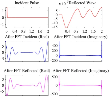
4.5 Software implementation of the inverse solver

The inversion scheme has already been tested to recon-struct sinusoidal shaped, square shaped and multiple Gaus-sian shaped relative permittivity profiles using the reflection data from Dirac pulse, Gaussian pulse, five pulses of sinu-soidal wave, raised cosine and step function in both noisy and noise free environment. A multiple Gaussian shapedεr

profile has been reconstructed here as an example simulation (see Figs. 9 and 10).

0 0.4 0.8 1.2 1.6 2 −1

0 1

Incident Pulse

0.4 0.8 1.2 1.6 2 −15

−10 −5 0 5

x 10 Reflected Wave−3

−5 0 5

After FFT Incident (Real)

−5 0 5

After FFT Reflected (Real) −200

0 200 400

After FFT Incident (Imaginary)

−500 0 500

After FFT Reflected (Imaginary)

Fig. 9. Incident wave, reflected wave and FFT results.L= 1_cm, Nz=Nx= 512,∆ = 1.95×10

−5

m,∆t= 85_ps.

5 Conclusions

The inverse solver presented in this paper shows almost accu-rate reconstruction. Better output can be geneaccu-rated by using higher resolutions. The tested resolutions are 128, 256, 512, 1024 and 2048. Besides all the combinations of relative per-mittivity and incident pulses have already been checked with synthetic and measured data. From the recent observations it has been proved that the inverse solver shows satisfactory

1 2

Original Permitivity Profile

1 2

Reconstructed Permitivity Profile

0.002 0.004 0.006 0.008 0.01 1

1.5 2 2.5

z in m −>

Red: Original Profile , Blue: Reconstructed Profile

Fig. 10. Top: Original profile; Middle: Reconstructed profile;

Bot-tom: Superposition of original and reconstructed profile.

result under noisy environment, too. Further modifications of the inversion algorithm are still going on. The next step is to reconstruct the permittivity and conductivity profiles from reflection and transmission data in lossy case.

References

Connor, K. M. and Dowding, C. H.: GeoMeasurements by Pulsing TDR Cables and Probes, CRC Press, Boca Raton, USA, 1999. Schlaeger, S.: Inveriosn of TDR Measurements to Reconstruct

Spa-tially Distributed Geophysical Ground Parameter, Ph.D. Thesis, Karlsruhe, Germany, 2002 (in German).

Taflove, A. and Hagness, S. C.: Computational Electrodynamics: The Finite-Difference Time-Domain Method, 2nd ed., Artech House, Boston, 2000.

Marklein, R.: The Finite Integration Technique as a General Tool to Compute Acoustic, Electromagnetic, Elastodynamic, and Cou-pled Wave Fields, in W. R. Stone (ed.), Review of Radio Science: 1999-2002 URSI, IEEE Press, Piscataway, 201-244, 2002. Krueger, R. J. and Ochs Jr., R. L.: A Green’s function approach to

the determination of internal fields, Applied Mathematical Sci-ences, 11, 525-543, 1989.

Corones, J. P., Davison, M. E. and Krueger, R. J.: Wave splittings, invariant embedding and inverse scattering, Inverse Optics, Proc. SPIE, 413, 102-106, 1983.

Kristensson, G. and Krueger, R. J.: Direct and inverse scattering in the time domain for a dissipative wave equation. Part 1 and Part 2, Journal of Mathematical Physics, 27, 1667-1693, 1986. Kristensson, G. and Krueger, R. J.: Direct and inverse scattering in

the time domain for a dissipative wave equation. Part 3: Scatter-ing operators in presence of phase velocity mismatch, Journal of Mathematical Physics, 28, 360-370, 1987.

Fig. 9. Incident wave, reflected wave and FFT results. L=1 cm,

Nz=Nx=512,1=1.95×10−5m,1t=85 ps.

The reconstruction is done in two steps as shown in in Fig. 8. At first,A(xi)is calculated from (i−1)-th grid. Secondly

R_i,j+ is calculated from current time step data of (i−1)-th grid, old time step data ofi-th grid and next time step data of

i−1-th grid.

4.5 Software implementation of the inverse solver

The inversion scheme has already been tested to recon-struct sinusoidal shaped, square shaped and multiple Gaus-sian shaped relative permittivity profiles using the reflection data from Dirac pulse, Gaussian pulse, five pulses of sinu-soidal wave, raised cosine and step function in both noisy and noise free environment. A multiple Gaussian shapedεr

6 M. Rahman and R. Marklein: Computation and Reconstruction of One-Dimensional Profiles Again from Eq. (46),

Ai=−4R+i−1,1

1 +∆ 2 8 A

2 i−₁

. (63)

The error made in Eqs. (62) and (63) is of orderO(∆3₎_{. The}

initialization of the algorithm is made by assigning, R+

0,j=R+(0,2j∆) =lR+(2jl∆); j= 0,1, ..., N . (64) The reconstruction is done in two steps as shown in in Fig. 8. At first,A(xi)is calculated from(i−1)-th grid. Secondly R+i,j is calculated from current time step data of(i−1)-th grid, old time step data ofi-th grid and next time step data of i−1-th grid.

4.5 Software implementation of the inverse solver The inversion scheme has already been tested to recon-struct sinusoidal shaped, square shaped and multiple Gaus-sian shaped relative permittivity profiles using the reflection data from Dirac pulse, Gaussian pulse, five pulses of sinu-soidal wave, raised cosine and step function in both noisy and noise free environment. A multiple Gaussian shapedεr

0 0.4 0.8 1.2 1.6 2 −1

0 1

Incident Pulse

0.4 0.8 1.2 1.6 2 −15

−10 −5 0 5

x 10 Reflected Wave−3

−5 0 5

After FFT Incident (Real)

−5 0 5

After FFT Reflected (Real) −200

0 200 400

After FFT Incident (Imaginary)

−500 0 500

After FFT Reflected (Imaginary)

Fig. 9. Incident wave, reflected wave and FFT results.L= 1cm,

Nz=Nx= 512,∆ = 1.95×10 −5

m,∆t= 85ps.

5 Conclusions

The inverse solver presented in this paper shows almost accu-rate reconstruction. Better output can be geneaccu-rated by using higher resolutions. The tested resolutions are 128, 256, 512, 1024 and 2048. Besides all the combinations of relative per-mittivity and incident pulses have already been checked with synthetic and measured data. From the recent observations it has been proved that the inverse solver shows satisfactory

1 2

Original Permitivity Profile

1 2

Reconstructed Permitivity Profile

0.002 0.004 0.006 0.008 0.01 1

1.5 2 2.5

z in m −>

Red: Original Profile , Blue: Reconstructed Profile

Fig. 10. Top: Original profile; Middle: Reconstructed profile; Bot-tom: Superposition of original and reconstructed profile.