Sensitivity Analysis of Parameter Hanges in Nonlinear Hydraulic Control Systems (RESEARCH NOTE)

(1)

RESEARCH NOTE

SENSITIVITY ANALYSIS OF PARAMETER CHANGES IN

NONLINEAR HYDRAULIC CONTROL SYSTEMS

S. Farahat, H. Ajam

Department of Mechanical Engineering, University of Sistan and Baluchestan, Zahedan, Iran

(Received: June 22, 2004)

Abstract In this research, the sensitivity analysis is applied to an electrohydraulic servovalve which is a nonlinear system. This system sensitivity study differs from previous studies by considering the dynamic behaviour and nonlinearity of the system performance. Different sensitivity analysis methods are compared to each other by studying the sensitivity of the actuator piston velocity of above servovalve with respect to eighteen parameters. By using the best method among the above mentioned methods, the sensitivity of the state variables of the sample system have been studied.

Keywords Sensitivity Analysis – Nonlinear Systems – Hydraulic Control Systems.

ﺪﻴﻜﭼ ه

ﺖـﺳاهﺪـﺷلﺎـﻤﻋاﻲﻄﺧﺮﻴﻏﻲﻜﻴﻟورﺪﻴﺋوﺮﺘﻜﻟاﺮﻴﺷﻢﺘﺴﻴﺳﻚﻳيورﺮﺑﺖﻴﺳﺎﺴﺣﺰﻴﻟﺎﻧآ،ﻪﻟﺎﻘﻣﻦﻳارد

. ﻪـﻌﻟﺎﻄﻣ

ﻢﺘﺴﻴﺳﻲﻄﺧﺮﻴﻏوﻲﻜﻴﻣﺎﻨﻳددﺮﻜﻠﻤﻋورﺎﺘﻓرﻦﺘﻓﺮﮔﺮﻈﻧردﺮﻃﺎﺧﻪﺑﻢﺘﺴﻴﺳﺖﻴﺳﺎﺴﺣ

ﺖـﺳاتوﺎـﻔﺘﻣﻲـﻠﺒﻗتﺎﻌﻟﺎﻄﻣﺎﺑ

.

ﻣيﺎﻫشور

ﻪﺴـﻳﺎﻘﻣﻢﻫﺎﺑﺮﺘﻣارﺎﭘهﺪﺠﻫﻪﺑﺖﺒﺴﻧنﻮﺘﺴﻴﭘﺖﻋﺮﺳﻲﺳرﺮﺑوقﻮﻓﻢﺘﺴﻴﺳﺮﺑلﺎﻤﻋاﺎﺑﺖﻴﺳﺎﺴﺣﺰﻴﻟﺎﻧآﻒﻠﺘﺨ

ﺪﻧاهﺪﺷ

. راﺮـﻗﻲـﺳرﺮﺑدرﻮﻤﻗﻮﻓﻢﺘﺴﻴﺳﺖﻟﺎﺣيﺎﻫﺮﻴﻐﺘﻣﺖﻴﺳﺎﺴﺣ،هﺪﺷﺮﻛذيﺎﻫشورنﺎﻴﻣزاشورﻦﻳﺮﺘﻬﺑزاهدﺎﻔﺘﺳاﺎﺑ

ﺪﻧاﻪﺘﻓﺮﮔ

.

1. INTRODUCTION

Dynamic system can be characterized in several ways: in the time domain, in the frequency domain, or in terms of a performance index. There is evidently an adequate number of ways to define the sensitivity function of a dynamic system. The definition that is actually used depends on the form of the mathematical model as well as on the purpose of consideration. For example, if the system is represented by a transfer function, the

sensitivity will be defined on the basis of the parameter-induced change of the transfer function; whereas in case of a space representation, the natural basis of the sensitivity definition will be the parameter-induced change of the trajectory.

Thus, the sensitivity function can be classified into the following three categories [1]:

•Sensitivity function in the time domain,

•Sensitivity function in the frequency or

z-domain,

•Performance-index sensitivity.

(2)

Besides these sensitivity function, there are so-called sensitivity measures that are defined on the entirety of the sensitivity function, and, therefore, allow for a global characterization of the sensitivity by a single number. These Entirety measures are used as an index in this research. The oldest definition of sensitivity function was given by Bode [2]. This definition is based on the transfer function and was restricted to infinitesimal parameter deviation. In the sequel, Horowitz [3] gave a different interpretation of Bode’s sensitivity function and also used it with great success for the design of control systems in the frequency domain [4,5]. Perkins and Cruz [6] extended Bode’s sensitivity function in different direction, also establishing its significance for time domain consideration.

In connection with simulation on network analyzer and analog computers, the output sensitivity functions were introduced in the fifties mainly by Bykhovsky [7] and Miller and Murray [8]. In the early sixties this definition was extended to the state space, resulting in the so-called trajectory sensitivity function [9,10,11]. The discussion of the merit of the time domain sensitivity function has not yet come to an end [4]. However, there is no doubt that they play an important role in the comparison of open- and closed-loop system as well as in the design of optimal controls. In 1963 Dorato [12] introduced the so-called performance-index sensitivity.

Beside the sensitivity function mentioned above there are various special sensitivity definitions, such as the sensitivity of the overshoot in the time or frequency domain, the eigenvalue (pole or zero) sensitivity, and so on. Definitions such as these may be very helpful in the characterization of the sensitivity of a system in a certain aspect such as its relative stability.

2. BASIC THEORY

Nonlinearities in the system models of

electro-hydraulic control servos complicate the application of the sensitivity analysis.The basis for the first order sensitivity models that can be applied to electro-hydraulic position control servos can be introduced as follow [13]:

)

,

(

x

u

α

f

x

&

=

v

(1)

where

x

is n-dimensional state vector

u is the r-dimensional input vector

α is the p-dimensional parameter vector It is assumed that unique solution of (1) exists for

all initial conditions and for all values of α.

Furthermore, it is assumed that

f

is continuously

twice differentiable with respect to

x

andα. Denote the nominal solution of equation (1):

)

,

(

)

(

_n

n

t

x

=

ϕ

α

(2)

where is the nominal value (subscript n

referring to nominal values) of

n

α

α. Denote the vector sensitivity function:

n j

x

⎟

⎠

⎞

⎜

⎝

⎛

∂

=

α

j

λ

j =1 … p (3)

Assuming that u is independent of α and

differentiating equation (1) partially with respect to

α

we obtain the sensitivity equation in the form:

n j j n j

f

x

f

⎟

⎠

⎞

⎜

⎝

⎛

∂

+

⎟⎟

⎠

⎞

⎜⎜

⎝

⎛

∂

=

α

λ

&

j =1 … p (4)

where (∂f/∂x) n is the Jacobian matrix evaluated on

the nominal solution.

The initial condition for (3) are :

j = 1 … p n j j

x

⎟

⎠

⎞

⎜

⎝

⎛

∂

=

α

λ

0

0 (5)

=

where x₀

ϕ

(

t

₀

,

α

_n

)

is the initial condition of

(3)

The sensitivity equations of (4) are linear differential equation with time-varying coefficient. There will be n(p+1) equation (n state variable

equations and n×p sensitivity equations) to be

(4)

solved to produce the system states and the sensitivity function. These equations can be solved using a computer simulation.

In the system models of electro-hydraulic control

servos the function f is continuous everywhere.

On the other hand, in the corner of some nonlinearity its first derivative is discontinuous.

Between these discontinuity points, f is

continuously twice differentiable with respect to and

x

.

α

So in the intermediate areas the

sensitivity equation can be defined in the form of (4). In solving the vector sensitivity functions one has to change the form of the

state function and sensitivity equations as one moves from one area to another. On the other hand, in the new area the initial condition of the altered equations are replaced by the final condition of the previous area.In the computer simulation this is done simply by the control logic, which recognizes the area in which we operate during the solution, and in moving from one area to another the structure of the state function and sensitivity equations is changed automatically to represent the conditions in the new area. So the initial conditions of the equations in the new area automatically given the values of the final conditions in the previous area. In the sensitivity model of this case, parameter influence on the discontinuity of the first derivate is not taken into consideration.

In addition to the sensitivity function, the complete differential variation of the nominal solution (2), which is:

)

,

(

)

,

(

α

ϕ

α

ϕ

δ

x

t

=

t

n

−

t

(6)

has to be known, and is due to the parameter variation:

n

α

δ

=

−

(7)

using Taylor's theorem, equation (6) may be written:

α

δ

α

δ

n

x

⎟

⎠

⎞

⎜

⎝

⎛

∂

=

+ higher order terms (8)

where (∂x /∂

α

)n is the n p matrix of the

sensitivity functions. The vector sensitivity functions are the columns of the sensitivity matrix. Once the vector sensitivity function have been known, according to equation (8), the first order

approximation of the variation δx can be

calculated.

×

3. VILENIUS METHOD

This method was introduced by Professor M.J. Vilenius [13] and has been applied to an electro-hydraulic position control servo. The main idea in this method is that, once one knows the size of the parameter variation δα, one is able to calculate the size of the variation of the nominal step response

of xi by only taking into account the first order

terms in equation (8) as follows:

∑

= = p j j j i i x 1

δα

λ

δ

i=1 … n ₍₉₎

With equation (9) we are able to calculate the size of any influence of parameter variation on the step response of xi at every time instant. To simplify the

comparison between the different parameters, equation (9) can be scaled with the steady state

value and consider only the maximum values of

δxi /xis and also change one parameter at a time.

Thus the equation for comparison will be as follows: is j j i j is i

x

λ

δα

δ

_max

max

=

(10)

By means of simulation studies it has been found [13] that the first order sensitivity model is still very accurate when the variations in the parameter

vector α are 10 percent. By comparison, Daniels,

(5)

and taking the maximum values according

to simulation programs, the maximum variations

can be computed by equation

(10). max j i

λ

j is i

x

max

δ

3. REVISED VILENIUS METHODS

This method is the same as the first method except that instead of computing δx i / δx is where xis is

the steady state step size,one should calculate

δxi(t)/xi(t) instantaneously, and then capture the

maximum value. This gives a better index comparison. Note that:

∑

=

p j j j i i

t

x

1

)

(

λ

δα

δ

then, (11)

∑

= = p j j i j i j i t x t t x t x

1 ( )

) ( )

( )

(

λ

δα

δ

Consequently, it is sufficient to compute

j = 1 to p

)

(

)

(

1 1

t

x

t

j

λ

(

)

(

2 2

t

x

t

j

λ

j = 1 to p

. . .

and then capture the maximum in each case. The only problem which remain yet, is the calculation of δx i (t)/xi (t) when x i (t) ≈0.0 .

To overcome this problem we can consider only the case where

x

i > ξxis where ξ can be 0 <ξ< 1.0 .

4. INDIVIDUAL CHARACTERISTICS METHOD

As it was mentioned in the first two methods, they choose only λij at one instant of the time, which is

the maximum in one or the other way. This λij not

only does not have information about other instants of the time but also its information at that special point of time is combination of different characteristics of the system performance changes (e.g. amplitude, frequency, …changes).

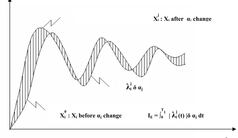
To make these problems more clear, the system performances before and after change of parameter

αj are presented in Figure.1. Amplitude differences

between the two curves at different points of times show the λijδαj, values. As it can be seen at some

points this value (λijδαj) is equal to zero. But it

dose not mean that the parameter change has no effect on the system performance rather, it means different characteristics changes of the system performance neutralize effects of each other at that point of time. Hence it will be better to study individual characteristics of the system performance separately.

5. ENTIRETY-INDEX METHOD

As it noticed, the different methods for the sensitivity analysis (methods 2-4) have various advantages and disadvantages. Individual characteristics method gives most of the system performance properties but it makes it difficult to use directly these result for some special purpose such as system optimization, and insensitivity. Then a simple method which has all or most of the system performance characteristics sensitivity has to be introduced.

For this purpose instead of capturing maximum

value of sensitivity, we integrate , over

some period of time (0:T1), figure 1. The integral

of j j iδα λ j j iδα

λ simply represent the area between two

state variable of the system.

6. SAMPLE SYSTEM

To apply the sensitivity analysis a novel electro-hydraulic servovalve has been chosen [15]. Considering a conventional hydraulic servovalve circuit instead of connecting backpressure of

(6)

actuator to drain through servo-valve, it will be connected to drain through a metering valve and a

Figure 1. Entirty Index of state variable Xi

t Xj

Xi 0

: Xi before αj change IE = ∫0 T1

|

λ

i j

(t) |δαj dt

λ

i j

δαj

Xi j

: Xiafter αjchange

relief valve (Figure. 2). In this way the backpressure and drain orifice area are controllable.

The system is defined by state model as below:

)

,

(

x

u

f

x

&

=

where x =

{

a_v,p₁,p₂,u_p

}

Using the informal equation of the various

components of the system, the function

f

can be

derived as bellow:

(

)

(

)

(

)

_⎪⎪⎪ ⎪ ⎪ ⎭ ⎪⎪ ⎪ ⎪ ⎪ ⎬ ⎫ ⎪ ⎪ ⎪ ⎪ ⎪ ⎩ ⎪⎪ ⎪ ⎪ ⎪ ⎨ ⎧ − − = = − + + − = = − − − = = + − − = = = M F A x x dt u d x x x c x A q v dt p d x x x c x A q v dt p d x in V a K v K x K v x f K a K v K x K v x v dt a d x u x f f p p p r p s v / ) ( ) ( ) ( 1 4 1 1 ) , ( 3 2 4 3 2 1 4 2 2 3 3 2 1 4 1 1 2 1 1 & & & & β β τ τ τ

Where q1,q2 (oil flows) and (supply, return

oil volume) depend on position of the direction

control valve which is controlled by input error voltage

r s

v

,

)

(Vi−Vf and (friction force ) depends

on x

f

F

4 (actuator piston velocity). Other parameter

defination and their values are given at the end.

7. APPLICATION OF THE METHODS

Four different methods are applied to the chosen hydraulic system and the best index selected. To compare different methods, only sensitivity of the state variable up which is most important output of

the system is considerd. But to study the sensitivity of other state variables the last method (entirety-index) is used to derive their sensitivity histograms with respect to all parameters change.

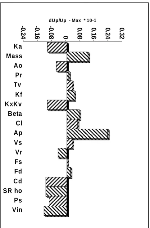
In the first method the ratio of the maximum

change of amplitude of state variable to

steady state value of amplitude of state variable is

(7)

studied, For example, for the last state variable (up)

with respect to first parameter (Ka); this ratio is as Kf

up

Ff

Fsum

Feedback

Transducer _{Actuator and}

Load

p1

q1

p2

q2

On - Off Controller

Ka

Servovalve Amplifier Vf

_

+ Vi

av

Ao Pr

Ps

International Journal of Engineering Vol. 18, No. 3, August 2005 -7

(8)

-0

.2

4

-0

.1

6

-0

.0

8 0

0.

0

8

0.

1

6

0.

2

4

0.

3

2

dU p/U p - Max * 10-1

Ka Mass Ao Pr Tv

Kf KxKv Beta Cl Ap Vs Vr Fs Fd Cd SR ho Ps Vin

Figure 3. Vilenius Method Histograms

below:

max max

4 1 1

4

) (

ps a a p

s U

K K

t u

x

t ⎟⎟⎠δ

⎞ ⎜⎜

⎝ ⎛

∂ ∂ = δα λ

The value of δα_j is 0.01α_j for all the histograms.

The time when these maximum changes of amplitudes occur, are approximately equal to the

peak-time (tp = 0.024 s; where up = Upmax). The

difference between these times and peak time depends on the individual characteristics changes

of state variable, especially rise time (Tr) and

frequency (Fr) changes. The value of these maxima

depends mostly on the steady state (Xss) and the

overshoot (Po) changes.

As the histogram of figure.1 indicate, the most

sensitive parameter is Ap and the insensitive

parameter is Fs some other relativity sensitive

parameters are Vin , Cd ,

1

/

ρ

, M , K a , KxKv

and Ps respectively. Two special parameters A o

and Pr which this sample system has been designed

according to them, are not as sensitive as other parameters.

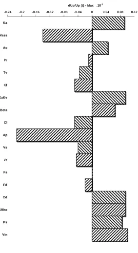
In the second method the maximum amplitude changes are considered with respect to the

performance value, up, at the same instant of time

(9)

max max 4 1 1 4

)

(

)

(

)

(

ps a a p s

U

K

t

u

t

x

t

δα

δ

λ

⎟⎟

⎠

⎞

⎜⎜

⎝

⎛

∂

=

But unlike the previous method which does not care for the value of the state variable in the time when maximum of λjiδαi occurs, this methods has

a tendency to choose the maximum of δλjiαij where

the state variable value is less than its steady state value. Hence the sign of the most sensitivity indices with respect to each parameter change are different in two histograms (figure.4). The same as

the pervious method, Ap is the most sensitive

parameter and Fs is the insensitive parameter. The

difference between the two methods is that the absolute values of all sensitivity indices change a

few percentages, except the absolute value of

∂

u

p/

∂

M index which increases about 33%. The

difference between this parameter (mass) and others is that according to the next method (individual characteristics) mass is the only parameter which is sensitive according to all individual characteristics and absolutely insensitive according to the steady state value.

The third method is the most detailed method considers different characteristics individually. Using the analytical method, the sensitivity of the five different characteristics (xss, Tr , Po ,Fr , Dc ) of

performance, up are evaluated. As it can be see

from the histogram (Figure. 5), each parameter has different effect on various characteristics. It is difficult to recognize this difference by using other methods. General survey of all the five histograms show that, as usual, Fs is insensitive Vin and Ap is

one of the most sensitive parameter, according to all performance characteristics, although in the two

pervious methods Vin was not as sensitive as Ap.

Sensitivity of the parameter in some performance characteristics such as the frequency surpasses the sensitivity of other parameters even parameter Ap .

This means that the sensitivity of the parameter

Vin according to different performance

characteristics somewhat nullify each other. Another interesting point is that in different histogram the order of the sensitivity of the parameter are different. For example in the first

histogram (Xss), Vin Cd and

1

/

ρ

are the most

sensitive parameters and Fs, Vr , Vs , β, τv , and

mass are absolutely insensitive parameters,

although in second histogram (Tr), mass is one of

most sensitive parameters (third one) and Cd and

ρ

/

1

almost insensitive parameters.

Entirety-Index Method gives an index (I=

∫

T

λ

jt

δα

_j

dt

0 ) (

4 )

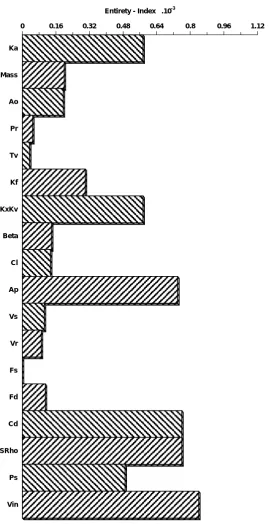
which is good combination of all the performance characteristics sensitivity with respect to each parameter. So it makes very easy to locate to an insensitive system. Unlike other methods, in this method we have only the absolute value of the sensitivity and it does not show that this sensitivity whether improves or deteriorates the performance. As it can be seen in histogram (Figure. 6)

parameters Vin , Cd ,

1

/

ρ

, Ap , Ka , and KxK v

which cause the most sensitivity on all the performance characteristics also are most sensitive

parameters in this method and Fs which was

insensitive parameter in all previous methods according to all performance characteristics, also is insensitive in this method. Other parameters have also a sensitivity which is combination of all different performance characteristics sensitivity with respect to that parameter.

8. CONCLUSION

A survey of all method shows that sensitivity parameters Ka and KxK v on the one hand and also

parameters Cd and

1

/

ρ

on the other are the same

according to all the methods and performance characteristics. This is because they appear in all the expression of simulation in the same position. Therefore it is possible to consider Ka× KxK v and

Cd×

1

/

ρ

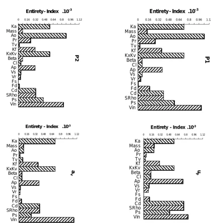
as combination parameters.

As it was mentioned the Entirety-Index is the best method, among four mentioned methods, for general optimization methods which consider all the performance characteristics together. Hence for this method all the four state variable are considered (Figure. 7). The effect of the parameters on sensitivity of the state variables av

and up are the same except that Ap and Cd

(also

1

/

ρ

) are among the most sensitive

(10)

Figure 4. Revised Vilenius Method Histograms

-0.24 -0.2 -0.16 -0.12 -0.08 -0.04 0 0.04 0.08 0.12 dUp/Up (t) - Max .10-1

Ka

Mass

Ao

Pr

Tv

Kf

KxKv

Beta

Cl

Ap

Vs

Vr

Fs

Fd

Cd

SRho

Ps

(11)

Figure 5. Individual Characteristic Method Histograms. -0.8 -0.7 -0.6 -0.5 -0.4 -0.3 -0.2 -0.1 0 0.1 0.2 0.3 0.4 0.5 0.6

Xss .10-1 Tr .10-3 Po .10-1

Fr Dc

Ka

Mass

Ao

Pr

Tv

Kf

KxKv

Beta

Cl

Ap

Vs

Vr

Fs

Fd

Cd

SRho

Ps

Vin

Xs

s

Tr

Po

Fr

Dc

(12)

0 0.16 0.32 0.48 0.64 0.8 0.96 1.12 Entirety - Index .10-3

Ka

Mass

Ao

Pr

Tv

Kf

KxKv

Beta

Cl

Ap

Vs

Vr

Fs

Fd

Cd

SRho

Ps

Vin

u

p

Figure 6. Entierty-Index Method Histogram up

(13)

0 0.16 0.32 0.48 0.64 0.8 0.96 1.12

Entirety - Index .10-3

Ka Mass Ao Pr Tv Kf KxKv Beta Cl Ap Vs Vr Fs Fd Cd SRho Ps Vin

P2

0 0.16 0.32 0.48 0.64 0.8 0.96 1.12

Entirety - Index .10-3

a

v

0 0.16 0.32 0.48 0.64 0.8 0.96 1.12

P1

0 0.16 0.32 0.48 0.64 0.8 0.96 1.12

u

p

Figure 7.Entierty-Index Method Histogram

p

₁,

p

₂,

a

_v, u_p

parameters of state variable up , but they are

among the least sensitive parameters of state variable av .

Although in actuator pressures (p1and p2), the

sensitivity of parameters Ap and Cd are low too,

parameter Ao which was one of the least sensitive

parameter (w.r.t up and av) is the most sensitive

parameter (w.r.t p1 and p2) even more sensitive

than parameter Vin . Also p1 about 20% more

sensitive than p2 to all the parameters except for

two. The first one is the parameter β (bulk

modulus of the oil) to which both pressure have the

(14)

same sensitivity, and the second one is the

parameter Fd (dynamic friction) to which pressure

p1 is ten times more sensitive than pressure p2.

9. SYSTEM PARAMETERS AND THEIR VALUES

Ao (orifice opernning of metering valve)

=2.066E-06(m2).

Ap (actutor pistonarea) =6.340E- 04(m2).

av (servovalve opening)

Cd (flow discharge coefficient) =6.000E-01

Fd (dynamic coulomb friction) =1.740E+02(N).

Fs (static coulomb friction) =4.500E+02(N).

Ka (servovalve amplifier gain)

=1.000E+01(mA/V).

Kf (velocity feedback gain) =9.000E+00(V/m/s).

Kx (servovalve torque motor constant (m/mA)).

Kv (servovalve area constant (m2/m)).

KxKv =8.325E-08(m2/mA).

M (total mass in motion) =8.400E+01(Kg). Ps (supply pressure ) =4.826E+06(N/m2).

Pr (relief valve setting pressure)

=4.826E+05(N/m2).

td (delay of direction control valve ) =8.000E-03(s).

T (period of square wave input signal) =4.000E-01(s).

vs (supply oil volume)

vr (return oil volume)

V 0 (piston referance velocity) =1.000E-04(m/s).

Vin (input signal voltag) =2.150E+00(Volt).

β (bulk moodulus of fluid ) =7.995E+09(N/m2).

ρ (density of the oil) =8.580E+02(Kg/m3).

τv (servovalve time constant) =4.000E-03(s).

10. REFERENCES

1. Frank, P.M., " Introducction to System

Sensitivity Theory ", Academic Press, New York, 1978.

2. Bode, H.W., "Network Analysis and Feedback

Amplifier Design." D. Van Nostrand Company NewYork 1945.

3. Horowitz, I.M., " Synthesis of Feedback

Systems. " Academic Press, New York, 1963.

4. Holtzman, J. M., and Horning S., "The

Sensitivity of Terminal Conditions of Optimal Control Systems to Parameter Variations ", IEEE Trans. Autom. Contr. Vol. 10. pp 420-426, 1965

5. Horowitz, I.M., and Shaked, U., " Superiosity

of Transfer Function over State Variable Methods in Linear Time- Invariant Feedback System Design " . IEEE Trans . Autom. Contr. Vol. 20, pp 84 - 97, Feb. 1975.

6. Perkins , W.R., and Cruz , J.B., "Sensitivity Operators for Linear Time - Varing Systems " , Proc. Int. Symp.Sensitivity , Dubrovink , Yugoslavia , 1964 , PP. 66-77. Pergamon Press, Oxford, 1966.

7. Bykhovskiy, M.L., " Sensitivity and Dynamic

Accuracy of Control Systems ", Eng. Cybern. USSR, pp 121 - 134, 1964. Reprinted in " System Sensitivity Analysis ", by Curz, J.B.

8. Miller, K. S., and Murray, F.J., " A

Mathematical Basis for the Error Analysis of Differential Analyzers ", J. Math. Phys. Cambridge, Mass., Vol. 32, pp 136 - 163, July - oct. 1953 .

9. Cruz, J.B. and Perkins, W.R., " A New

Approach to the Sensitivity Problem in Multivarible Feedback Systems Design " , IEEE Trans. Autom. Contr. Vol. 9, pp 216 - 233, July 1964 .

10.Randavic, L., " Sensitivity Methods in Control Theory ", Proc. Int. Sump. Sensitivity, Dubrovnik, Yugoslavia , 1964. Pergamon Press, Oxford, 1966.

11.Tomovic, R., " Sensitivity Analysis of

Dynamic Systems. " McGraw -Hill, New York, 1963.

12.Dorato, P., " On Sensitivity in Optimal Control Systems ", IEEE Trans. Autom. Contr. Vol. 8, pp 256 -257, July 1963.

(15)

Sensitivity Analysis to Electrohydraulic Position Control Servos. " , ASME Journal of Dynamic Systems , Mesurment and Control , Vol . 105, June 1983, pp 77 - 82.

14.Daniels, A.R., Lee, Y.B., and Pal, M.K.,

"Nonlinear Power - Systems Optimization Using Dynamic Sensitivity Analysis ," Proceedings of IEE, Vol . 123, No.4 , April

1976, pp 365 - 370.

15. Limaye A.M., " Design and Development of a Novel Electro - Hydraulic Servovalve Configuration " As a Master of Engineering Thesis at Mechanical Engineering Department of Concordia University , Montreal, Quebec, Canada . 1985