Analytical approximate solution of higher order boundary value problems via variational iteration method

(1)

BIBECHANA

A Multidisciplinary Journal of Science, Technology and Mathematics

ISSN 2091-0762 (Print), 2382-5340 (0nline)

Journal homepage: http://nepjol.info/index.php/BIBECHANA

Publisher: Research Council of Science and Technology, Biratnagar, Nepal

Analytical approximate solution of higher order boundary value

problems via variational iteration method

Zobia Hamid, Jamshad Ahmad*

Department of Mathematics, Faculty of Science, University of Gujrat, Pakistan.

*_Email:

_{[email protected]}

Article history: Received 09 October, 2017; Accepted 31 October, 2017

DOI: http://dx.doi.org/10.3126/bibechana.v15i0.18347

This work is licensed under the Creative Commons CC BY-NC License. https://creativecommons.org/licenses/by-nc/4.0/

Abstract

In this paper, application of variational iteration method has been successfully extended to obtain approximate solutions of some higher order boundary value problems. We emphasize the power of the method by testing three different mathematical models of distinct orders. The results are obtained by using only little iteration.

Keywords: Nonlinear BVP;Variational iteration method; Approximate solution.

1. Introduction

(2)

2. The Analysis of Variational Iteration Method

Consider the general differential equation

Lu+Nu = g(x) (1)

where L and N are linear and nonlinear operators respectively, and g(x) is the source inhomogeneous term. The variational iteration method admits the use of a correction functional for equation (1) in the form

, dt )) t ( g ) t ( u N ) t ( Lu ( ) t ( ) x ( u ) x (

u _n n

x

0 n 1

n     



 (2)

where



is a general Lagrange’s multiplier, which can be identified optimally via the variational theory, and 𝑢̅̅̅̅𝑛 as a restricted variation which means 𝛿𝑢̅̅̅̅𝑛 =0. The Lagrange multiplier



is crucial and critical in the method, and it can be a constant or a function. Having



determined, an iteration

formula should be used for the determination of the successive approximations

u

n1

(

x

)

;

n



0

of the solution u(x). The zeroth approximation u0 can be any selective function. However, using the initial

values u(0);u(0); and u(0) are preferably used for the selective zeroth approximation

u

₀ as will

be seen later. Consequently, the solution is given by

) x ( u Lim ) x (

u _n

n

 (3)

3. Numerical Applications

Problem 3.1 Consider a fifth order non-linear BVP

( )v _{( )} x ( )ii _{( ),}

u x e u x (4)

with boundary conditions

(0) (0) (0) 1 , (1) (1) 1.

u u u  u u  (5)

The correctional functional is given as

, dt )} t ( u e ) t ( u { ) x ( u ) x ( u

x

0

) ii ( n t ) v ( n n

1

n   



 (6)

where ‘λ’ is langrage multiplier, which is identified as

1 ( 1) ( )

.

( 1)

m m

t x

m









 





(7)

And the initial approximation is 0( ) ,

x

e x

u 

For n=0,the equation (6) gives,

, dt )} t ( u e ) t ( u { ) x t ( 24

1 ) x ( u ) x (

u ₀(5) t ₀(ii)

x

0 4 0

1



  





(t x) (e 1)dt, 24

1

e t

x

0 4

x _ _{ } _



120 x 24 x 6 x 2 x x 1

5 4 3 2

     

For n=1,

, dt )} t ( u e ) t ( u { ) x t ( 24

1 ) x ( u ) x (

u x ₁(5) t ₁(ii)

0 4 1

2



  

 



, x 2 21 e 56 xe 21 e x 3 e 6 x x 34 2 x 3 24

x 5

57 x 2 x x x 2

3 3

4

 

 

  

(3)

The approximate solution is

14 11 13

10 12

9

11 8 10

9 6

8 7

6 5 4 3

2

n

x 10 558747 1470745608 .

1 x 10 333186 6059043833 .

1 x 10 86751 0876756987 .

2

x 10 44172 5052108385 .

2 2628800

x x 10 9966 7557319236 .

2

x 0000248016 .

0 5040

x 720

x 120

x x 0416667 . 0 x 166667 . 0 2 x x 1 ) x ( u

 



 

 



 

 



 

   

   

Fig 1: Comparison of exact and approximate solution.

Problem 3.2 Consider a non-linear BVP

( ) 2

( )

( ),

vi x

u

x



e u x

(8)

1 1 1

(0) 1, (0) 1, (0) 1, (1) , (1) , (1) .

u  u   u  u e u  e u e (9)

The correctional functional is given as

( ) ( )

1

0

( ) ( ) { ( ) ( )} ,

x

v x ii

n n n n

u _ x u x 



 u t e u t dt (10)

where ‘λ’ is langrage multiplier ,which is calculated by

1 5

( 1) ( ) ( )

,

( 1) 5

m m

t x t x

m



 



 

  

 

 (11)

And the initial approximation is

, e ) x ( u₀  x

(12) For n=0, the equation (10) becomes,

dt ))} t ( u ( e ) t ( u { ) x t ( 120

1 ) x ( u ) x (

u x _o(vi) t ₀(ii)

0 5 0

1      ,

(t x) {e e (e )}dt 120

1

e t t t

x

0 5

x  

 _

  

 ,

  

 

        

5 x 4 x 3 x 2 x x 1

5 4 3 2

,

Closed

Ap p roximate

2 2 4 6 8

(4)

dt ))} t ( u ( e ) t ( u { ) x t ( 120 1 ) x ( u ) x (

u ₁(vi) t ₁(ii)

x

0 5 1

2      ,

209 20 x x 12 7 x 6 x 2 69 xe 84 24 e x e x 6 7 e x 14 x 127 e 210 5 4 3 2 x x 4 x 3 x 2

x_ _ _ _ _ _ _ _ _ _





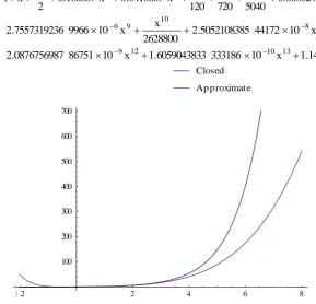
                          14 11 13 10 12 9 11 8 10 7 8 7 6 5 4 3 2 x 10 729725 1470745597 . 1 x 10 6059043836 . 1 x 10 868175 0876756987 . 2 x 10 56 5052108667 . 2 x 10 76053 7557319336 . 2 40320 x 5040 x 720 x x 0083333 . 0 x 0416667 . 0 x 166667 . 0 2 x x 1 ) x ( u

The closed solution of this problem is e-x _.

Fig.2: Comparison of closed and approximate solution.

Problem 3.3 Consider a six order non-linear BVP

) x ( u e

u(vi) x (ii) (13) with boundary conditions

1 ) 0 ( u ) 0 ( u ) 0 (

u    (iv)  (14)

e ) 1 ( u ) 1 ( u ) 1 (

u    (iv)  (15) The correctional functional is given as

, dt )} t ( u e ) t ( u { ) x ( u ) x ( u x 0 ) ii ( n t ) vi ( n n 1

n   



 (16)

where ‘λ’ is langrage multiplier, which is identified as

; 5 ) x t ( ) 1 m ( ) x t ( ) 1

( m m 1 5

          

 (17)

And the initial approximation is

, ) ( 0 x e x u  (18) For n=0,the equation (17) becomes,

, dt )} e ( e e { ) x t ( 120 1 e ) x (

u t t t

x 0 5 x 1      

6 4 2 2 4

50 100 150

Closed

(5)

   

 

          

6 x 5 x 4 x 3 x 2 x x 1

6 5 4 3 2

, dt )} t ( u e ) t ( u { ) x t ( 120

1 ) x ( u ) x (

u ₁(vi) t ₁

x

0 5 1

2      



4

2 3 2 3

4 5

7 69

127 210 84 14 6

6 24 2

7 1

12 20

x

x x x x x e

x e xe x e x e x x

x x



   

        



14 11 13

10 12

9

11 8 10

7 9

6

8 7

6 5 4

3 2

x 10 1470745597 .

1 x 10 6059043867 .

1 x 10 0876756988 .

2

x 10 5052109648 .

2 x 10 7557319224 .

2 x 10 7557318996 .

2

x 0000248016 .

0 x 000198413 .

0 720

x x 00833333 .

0 24 x x 166667 . 0 2 x x 1 ) x ( u

 



 



 



 



 

  

Fig.3: Comparison of exact and approximate solution.

4. Conclusion

In this work, the variational iteration method has been successfully employed on higher order boundary value problems by converting into corresponding system of first order differential equations. The obtained results are good agreement with the existing results in literature.

References

[1] A. M. Wazwaz, The variational iteration method for analytic treatment for linear and nonlinear ODEs, Appl. Math. Comput. 212 (2009) 120–134. doi.org/10.1016/j.amc.2009.02.003.

[2] M. Abolhasani, S. Abbasbandy, T. Allahviranloo, A New Variational Iteration Method for a Class of Fractional Convection-Diffusion Equations in Large Domains, Mathematics, 5 (2017) 26. doi.org/10.3390/math5020026.

[3] B. D. Yuliyanto, Variational iteration method for solving the population dynamics model of two species, IOP Conf. Series: J. Phys.: Conf. Ser. 795 (2017) 012044.

doi.org/10.1088/1742-6596/795/1/012044.

5 10 15

5000 10000 15000 20000 25000 30000 35000

Closed

(6)

[4] J. H. He, Variational iteration method for autonomous ordinary differential systems, Appl. Math. Comput. 114 (2000) 115–123. doi.org/10.1016/S0096-3003(99)00104-6.

[5] J. H. He, Variational iteration method - Some recent results and new interpretations, J. Comput. Appl. Math. 207 ( 2007) 3–17.

doi.org/

10.1016/j.cam.2006.07.009.

[6] M. Torvattanabun, S. Koonprasert, Variational Iteration Method for Solving Eighth-Order Boundary Value Problems, Thai J Math. (2010) 121–129.

[7] A. M. Wazwaz, The variational iteration method for solving linear and nonlinear ODEs and scientific models with variable coefficient, Cent. Eur. J. Eng. 4 (2014) 64-71. doi.org/10.2478/s13531-013-0141-6.uropean Journal of Engineering.

[8] M.T Akter, M.A.M Chowdhury, Variational Iteration Method for Solving Coupled Schrödinger-Klein-Gordon Equation, American J. Comput. Appl. Math. 7 (2017)

25-1. doi.org/10.5923/j.ajcam.20170701.03.

[9] K. N. S. K. Viswanadham, Numerical Solution of Ninth Order Boundary Value Problems by Petrov-Galerkin Method with Quintic B-splines as Basis Functions and Septic B-splines as Weight Functions, Procedia Eng. 127 (2015) 1227-1234. doi.org/10.1016/j.proeng.2015.11.470.

[10] R. P. Agarwal, Boundary Value Problems for High Ordinary Differential Equations, World Scientific, Singapore, 1986.

[11] S. T. Mohyud-Din, M.A Noor, K.I. Noor, Variation of Parameters Method for Solving a Class Of Eighth-Order Boundary-Value Problems, Int. J. Comput. Methods. 9 (2012) 1240026.

doi.org/10.1142/S0219876212400269.

[12] H. N. Caglar, S. H. Caglar, E.H. Twizell, The numerical solution of fifth-order boundary value problems with sixth degree B-spline functions, Appl. Math. Lett. 12 (1999) 25–30. doi.org/10.1016/S0893-9659(99)00052-X.

[13] A. M. Wazwaz, The numerical solution of fifth-order boundary value problems by the decomposition method, J. Comput. Appl. Math. 136 (2001) 259–270. doi.org/10.1016/S0377-0427(00)00618-X.

[14] E. H. Twizell, A. Boutayeb, Numerical methods for the solution of special and general sixth-order boundary value problems, with applications to B´enard layer eigenvalue problems, Proc. R. Soc. of Lond. A, 431 (1990) 433–450. doi.org/ 10.1098/rspa.1990.0142.

[15] A. M. Wazwaz, The numerical solution of sixth-order boundary value problems by the modified decomposition method, Appl. Math. Comput. 118 (2001) 311–325. doi.org/10.1016/S0096-3003(99)00224-6.

[17] I. Ullah, H. Khan, M.T. Rahim, Numerical solutions of higher order nonlinear boundary value problems by new iterative method, Appl. Math. Sci. 7 (2013) 2429–2439.