Computing Lower Bounds of µ-Values for a Class of Rotary Electrical Machines

(1)

Volume 17, Number 1 (2019), 33-46

URL:https://doi.org/10.28924/2291-8639 DOI:10.28924/2291-8639-17-2019-33

COMPUTING LOWER BOUNDS OF µ-VALUES FOR A CLASS OF ROTARY

ELECTRICAL MACHINES

MUTTI-UR REHMAN∗, M. FAZEEL ANWAR

Department of Mathematics, Sukkur IBA University, 65200 Sukkur-Pakistan

∗_{Corresponding author:} _{[email protected]}

Abstract. In this article we present the computations of lower bounds of well-known mathematical quantity in control theory known as structured singular value for a family of structured matrices obtained for a DC Motor, that is an electrical machine. The comparison of lower bounds with the well-known MATLAB function mussv is studied. The structured singular values provide an important tool to synthesize robustness as well as analyze performance and stability of feedback systems.

1. _Introduction

The Structured Singular Value (SSV) [1] is an important and versatile tool in system theory which allows

one to address a central problem in control systems i.e. to analyze the stability of a system. The class of

structures addressed by the SSV is very generic and covers almost all kinds of parametric perturbations that

can be incorporated into the control system via real or complex linear fractional transformations (LFTs).

We refer the interested readers to see [2 - 9] and the references there in for more examples and applications

of SSV.

The exact computations of SSV are NP hard [10]. There are however several algorithms available in

literature to compute lower and upper bounds for SSV. An upper bound of SSV guaranties the robust

stability, while the lower bounds of SSV provides information about instability of linear closed loop systems.

Received 2018-08-04; accepted 2018-10-06; published 2019-01-04. 2010Mathematics Subject Classification. 65F15, 34H05.

Key words and phrases. structured singular value; spectral value set; block diagonal uncertainties; spectral radius; low-rank matrix manifolds, gradient system of ODEs.

c

2019 Authors retain the copyrights of their papers, and all open access articles are distributed under the terms of the Creative Commons Attribution License.

(2)

The widely used routine, mussv, available in MATLAB control Toolbox approximates upper bound by

means of the diagonal balancing and linear matrix inequalities (LMI) techniques [11, 12]. While on the other

hand, lower bound is approximated by generalization of power method [13-14].

In this paper, we present numerical approximations to a lower bound of the SSV associated with mixed

real and complex uncertainties. Our approach is based on a two level algorithm, inner-outer algorithm, given

in [17].

2. _{Overview of the article}

Section 3 provides the basic framework of proposed problem. We explain how a better approximation of

the structured singular values can be obtained by a two level algorithm that is an inner-outer algorithm.

The outer algorithm determines the perturbation level while the inner algorithm computes the desired

perturbation. The inner algorithm then determines a (local) extremizer of the structured spectral value set.

In Section 4, we introduce the inner algorithm for the case of pure complex uncertainties. An important

characterization of extremizers help us to restrict the problem to a manifold of structured perturbations

with normalized and low-rank blocks. A gradient system of ODEs for finding extremizers on this manifold

is established. Finally, in Section 5, we give a range of numerical experiments to compare lower bounds of

SSV obtained with proposed algorithm [17] to those obtained with mussv.

3. _Framework

Let C = _C and R = _R and let Cn,n₍_Rn,n_{) denote the family of complex (real) matrices. For} _M _∈

Cn,n(Rn,n) we consider an underlying perturbation set with prescribed block diagonal matrices given below

B={diag(δiIi,∆j) :δi∈C(R),∆j∈Cn,n(Rn,n)}. (3.1)

The following definition is given in [1], where I is then×nidentity matrix.

Definition 3.1. LetM ∈Cn,n _{and ∆}_∈

Bis an admissible perturbation. Then structured singular value

ofM is denoted byµ_B(M) and is defined as follows

µ_B(M) := 1

min{k∆k2: ∆∈B,det(I−M∆) = 0}

. (3.2)

In above definition 3.2, det(·) represents the determinant of a matrix (I−M∆) while minimum is over an

admissible perturbation ∆.

For a general set Bthe SSV become smaller and thus we have an upper bound. The important special

case, when the set_Bonly consists of pure complex perturbations, we denote the set by_B∗instead of_B. For

∆∈B∗ we haveeiθ∆ ∈B for anyθ ∈R. As a result, this gives us a suitable choice of ∆∈∆B∗ such that

(3)

same matrix 2-norm so thatM∆0 possess an eigenvalue 1. This in turn implies that the matrixI−M∆0 is

singular. This gives us the following alternative definition of the SSV

µ_B∗(M) :==

1

min{k∆k2: ∆∈_B∗_{, ρ}₍_M_{∆) = 1}_}. (3.3)

In Equ. (3.3), ρ(·) denotes the spectral radius of a matrixM∆.

3.1. Overview of the proposed methodology. We need to solve the maximization problem

λ() =arg max|λ| (3.4)

where maximum is overλ for some fixed parameter >0. It is clear thatµ_B∗(M) is the reciprocal of the

smallest value offor whichλ() = 1. This suggests a two level algorithm. In the inner algorithm, we intend

to solve the problem addressed in Equ. (3.4). In the outer algorithm we first varyby using the fast Newtons

method and this exploits the knowledge of the computation of the exact derivative of the extremizers. We

address Equ. (3.4) by solving a system of ordinary differential equations.

4. Computation of local extremizers

In this section we present the inner algorithm for optimization problem addressed in Equ. (3.4). We use

the following standard eigenvalue perturbation result.

Lemma 4.1. [15]. Consider a family of matricesA :R→Cn,n and let λ(t) be an eigenvalue ofA(t) for

all values of t. The eigenvalue λ(t) tends to converge to the simple eigenvalueλ0=λ(0), ofA0 =A(0) as

t→0. Thereforλ(t) is analytic neart= 0 with

dλ(t) dt =

X₀∗BX0

X₀∗X0

where,X₀∗,X0are the left and right eigenvectors ofA0=A(0) associated with simple eigenvalueλ0=λ(0),

that is, X₀∗(A0−λ0I) = 0 and (A0−λ0I)X∗ = 0 and the matrix B is the time derivative of the matrix

valued functionA(t).

Definition 4.2. An admissible perturbation ∆∈B∗ such thatk∆k2≤1 and the matrix (M∆) for some

fixed parameter >0 has greatest eigenvalueλmaxwhich maximizes locally the modulus of ΛB ∗

(M) is known

as a local maximizer.

Theorem 4.3. Let

b

∆ ={diag(δiIi,∆j) :δi ∈C,∆j ∈Cmj,mj, ∀i= 1 :S, J= 1 :F} (4.1)

with k∆bk2 = 1 be a local extremizer. The matrix M∆ possesses the simple eigenvalueλ=|λ|eiθ, θ∈R,

with xand y being right and left eigenvectors for an eigenvalue λ. The eigenvectors are scaled such that

s=eiθ_y∗_{x >}_{0. Partitioning}_x_and_y_{according to size and structure of}

b

∆ yields

(4)

y= (y₁T, . . . , y_nT, y_nT₊₁, . . . , y_nT₊_F)T. (4.2)

Now we takez=M∗y= (zT1, . . . , znT, znT+1, . . . , znT+F)

T_{and assume the non-degeneracy conditions given}

by

z_k∗xk 6= 0 ∀k= 1, . . . , n, (4.3)

kzn+hk2· kxn+hk26= 0 ∀h= 1, . . . , F. (4.4)

Hence,

|δk|= 1 ∀k= 1, . . . , s and k∆k2= 1 ∀h= 1, . . . , F.

Theorem 4.4. Let

b

∆ ={diag(δiIi,∆j) :δi ∈C,∆j ∈Cmj,mj, ∀i= 1 :S, J= 1 :F} (4.5)

with k∆bk2 = 1 be a local extremizer. Suppose that λ, x, z are defined and partitioned as in Theorem 4.3.

Assume the non-degeneracy condition of (4.4) and every block possess a singular value which attains the

maximum value 1. Then the matrix,

b

∆ ={diag(δ1I1, ..., δsIs;u1v∗1, ..., uFv∗F)}

is a local extremizer.

Remark 4.5. Theorem 4.4 allows us to restrict the admissible perturbations in the structured spectral

value set given in (3.4) to those with rank-1 blocks. Since the Frobenius and the matrix 2-norms of a rank-1

matrix are same, this helps us to search for extremizers within the sub-manifold

B₁∗={diag(δ1I1; ∆j) :δi∈C,∆j∈Cmj,mj,∀i= 1 :S, j= 1 :F}. (4.6)

4.6. Approximating extremal points of ΛB∗ (M).

In order to approximate the local maxima for ΛB∗(M) we construct a matrix valued function ∆(t) where

∆(t)∈_B∗_{such that the largest eigenvalue}_λ_{of the matrix}_M_∆(_t_{) achieves the maximum (local) growth. We}

then derive a gradient system of ODEs which satisfies the choice of the initial matrix admissible perturbation

∆(t).

4.7. The local optimization problem.

We consider the fact thatλ=|λ|eiθ_{is the simple eigenvalue with the corresponding eigenvectors, normalized}

such that

kxk=kyk= 1, y∗x=|y∗x|e−iθ. (4.7)

As a result of the Lemma 4.1, we get the following expression for the change in the largest eigenvalue.

d dt|λ|

2₌ 2|λ| |y∗_x_|Re(z

(5)

The eigenvectors x and y are defined and normalized as in the Theorem 4.3. Now, by considering the

suitable perturbation ∆∈B₁∗ withB₁∗ in Equ. (4.6), we aim to determine a direction ∆∗=z that (locally)

maximizes the increase of the modulus of λ. This amounts to determining a direction Z as given in the

following equation

Z=diag(ω1Ir1, . . . , ωsIrN,Ω1, . . . ,ΩF) (4.9)

which is the solution of the following optimization problem

Z = arg max{Re(z∗Zx)}

subject to Re(δiωi) = 0, i= 1 :S,

and Reh∆j,Ωji= 0, j= 1 :F. (4.10)

The linear constraints in maximization problem in Equ. (4.10) ensure that Z lies in the tangent space of

the manifold B₁∗ at ∆(t). In particular Equ. (4.10) ensures that the norm of each block of the admissible

perturbation ∆(t) remain conserved.

Lemma 4.6. The solution of the maximization problem as discussed in (4.10) is given by

Z∗={diag(ω1Ir1, . . . , ωNIrN,Ω1, . . . ,ΩF)}, (4.11)

with

ωi = νi x∗izi−Re x∗iziδi

δi

, i= 1, . . . , S (4.12)

Ωj = ζj zs+jx∗N+j−Reh∆j, zs+jx∗s+ji∆j

, j = 1, . . . , F. (4.13)

Wherevi>0 andζj>0. If the right-hand sides are different from zero thenZ ∈B1∗.

Corollary 4.7. The result of the lemma 4.6 can be written as follows:

Z∗=D1P_B∗(zx∗)−D₂∆, (4.14)

whereP_B∗(·) is the orthogonal projection andD₁, D₂∈_B∗ are diagonal matrices withD₁ is positive.

4.8. The gradient system of ordinary differential equations.

Following Lemma 4.6 and Corollary 4.7 we consider the following differential equations on the manifold

B₁∗.

˙

∆ =D1PB∗(zx

∗₎₋_D

2∆. (4.15)

where, x(t) is an eigenvector associated to a simple eigenvalueλ(t) of the matrix M∆(t) for some fixed

> 0. Also note that the quantitiesz(t), D1 andD2 depend on the choice of the matrix valued function

(6)

4.9. Choice of initial value matrix and0.

In order to compute0we choose the initial value matrix

∆0=D P∆B(wv

∗₎_, _(4.16)

whereD is the positive diagonal matrix such that ∆0∈B∗. As a natural choice for the initialization of the

perturbation level, we take0 as

0=

1

b µ_B∗(M)

. (4.17)

whereµ_b_B∗(M) is the upper bound of µ-value approximated by mussv.

5. Numerical Testing

In this section we present various numerical experimentations for both pure and mixed real and complex

perturbations. The comparisons of lower bounds of structured singular values for a class of matrices obtained

for DC Motor are considered.

Example 1. Consider the following five dimensional matrix.

M =            

−.050−.113i −.012−.028i −.216 +.072i −.000−.000i 6.306−2.099i

.113−.050i .028−.012i −.072−.216i .000−.000i 2.099 + 6.306i

−.050−.113i −.012−.028i −.073 +.072i −.000−.000i 6.306−2.099i

−.004−.008i −.001−.002i .001 +.005i .142−.000i −.042−.153i

−.004−.008i −.001−.002i −.001−.002i −.000−.000i −.042−.153i             .

Also, consider the set of block diagonal uncertainties as an input argument. The uncertainty set is taken as

B={diag(δ1I2,∆1) :δ1∈R,∆1∈C3,3}.

Making use of MATLAB function mussv, we obtain an admissible perturbation set∆, which is given belowb

b ∆ =            

−.149 0 0 0 0

0 −.149 0 0 0

0 0 −.001−.001i 0 0

0 0 .000−.0001i 0 0

0 0 −.143−.044i −.0008 + 0.0033i −.0008 +.0033i             .

The 2-norm of admissible perturbation is obtained as 0.1499 while the lower bound of structured singular

value is obtained asµl

(7)

Applying the algorithm presented in article [17], we obtain the admissible uncertainty∇b with= 0.1499

and∇b with

b ∇=            

−1 0 0 0 0

0 −1 0 0 0

0 0 −0.0115−0.0100i 0.0002−0.0002i 0.0002−0.0002i

0 0 0.0001−0.0003i 0 0

0 0 −0.9541−0.2976i −0.0065 + 0.0207i −0.0070 + 0.0206i             .

In this case the admissible uncertainty has a unit 2-norm while the obtained lower bound of structured

singular value isµl_Our(M) = 6.6708.

M =            

−.169−.155i −.042−.038i −.176 +.137i −.000−.000i 5.136−3.998i

.310−.338i .077−.084i −.274−.352i .001−.001i 7.997 + 10.272i

−.169−.155i −.042−.038i −.033 +.137i −.000−.000i 5.136−3.998i

−.014−.008i −.003−.002i .005 +.009i .142−.000i −.168−.266i

−.014−.008i −.003−.002i .005−.009i .142−.000i −.168−.266i             .

B={diag(δ1I1,∆1) :δ1∈R,∆1∈C4,4}.

b ∆ =            

−0.0679 0 0 0 0

0 −.0004 +.0004i −.0002 +.0002i 0 0

0 −.0013 +.0014i −.0007−.0006i 0 0

0 0 0 0 0

0 .036−.048i −.024 +.018i −.0007 +.001i −.0007 +.001i             .

(8)

and∇b with

b ∇=            

−1 0 0 0 0

0 .005 +.005i −.002 +.002i −.0001−.0001i −.0001−.0001i

0 −.018 +.020i −.010−.009i .0004−.0005i .0004−.0005i

0 −.0001 +.0001i 0 0 0

0 .541 +.711i .355 +.270i −.0109 +.018i −.010 +.181i             .

M =            

−.283−.099i −.070−.024i −.109 +.178i −.001−.000i 3.195−5.200i

.299−.849i .074−.212i −.534−.328i .001−.003i 15.600 + 9.587i

−.283−.099i −.070−.024i −.033 +.178i −.001−.000i 3.195−5.200i

−.021−.001i −.005−.0003i .011 +.009i .142−.000i −.346−.286i

−.021−.001i −.005−.0003i .011 +.009i −.0001−.000 −.346−.286i             .

B={diag(δ1I1, δ2I1, δ3I1,∆1) :δ1, δ2, δ3∈R,∆1∈C2,2}.

b ∆ =            

−.586 + 1.067i 0 0 0 0

0 −.586 + 1.067i 0 0 0

0 0 −.586 + 1.067i 0 0

0 0 0 .109 .105

0 0 0 −.594 +.631i −.576 +.612i             .

(9)

and∇b with

b ∇=            

−.492 +.870 0 0 0 0

0 −.492 +.870 0 0 0

0 0 −.492 +.870 0 0

0 0 0 .087 +.0009i .085 +.001i

0 0 0 −.484 +.520i −.472 +.506i             .

M =            

−.326 +.009i −.081−.002i −.036 +.181i −.001−.000i 1.065−5.282i

−.038−1.306i −.009−.326i −.724−.146i −.0002−.005i 21.128 + 4.260i

−.326 +.009i −.081 +.002i .106 +.181i −.001 1.065−5.282i

−.020 +.009i −.005 + 0.002i .017 +.006i .142−.000i −.498−.196i

−.020 +.009i −.005 +.002i .017 +.006i −.0001−.000i −.498−0.196i             .

B={diag(δ1I1, δ2I1,∆1) :δ1, δ2,∈R,∆1∈C3,3}.

b ∆ =            

−.173 0 0 0 0

0 −.134 0 0 0

0 0 .002−.005i .0006 +.0002i .0006 +.0002i

0 0 −.0004i 0 0

0 0 .041 +.166i −.014 +.006i −.014 +.006i             .

(10)

and∇b with

b ∇=



          

−1 0 0 0 0

0 −.911 0 0 0

0 0 .015−.032i .003 +.0009i .003 +.0009i

0 0 .0002−.002i .0002 .0002

0 0 .247 +.959i −.083 +.038i −.083 +.038i 

           .

singular value isµl

Our(M) = 0.3709.

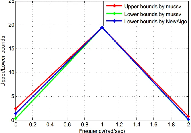
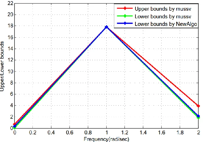
In each of following figure, we present the comparison of lower bounds of structured singular values obtained

by MATLAB routine mussv and the algorithm presented in [17], for five dimensional complex matrices. Each

of these matrix is computed from [16].

6. _Conclusion

In this article we have considered the problem for the computation of the lower bound of structured singular

values for a family of complex matrices obtained in [16]. The computation of structured singular values plays

an important role in robust stability and instability in control. The experimental results show the comparison

of the lower bounds computed by algorithm [17] when compared to well-known1 MATLAB function mussv

available in MATLAB Control toolbox.

7. _Nomenclature

B Family of block diagonal matrices

0 Perturbation level

∆0 Initial admissible perturbation

µ Structured Singular Values

References

[1] Packard, Andrew and Doyle, John. The complex structured singular value.Automatica, 29(1993): 71-109.

[2] Bernhardsson, Bo and Rantzer, Anders and Qiu, Li. Real perturbation values and real quadratic forms in a complex vector space.Linear Algebra Appl., 270(1998): 131-154.

[3] Chen, Jie and Fan, Michael KH and Nett, Carl N. Structured singular values with nondiagonal structures. I. Characteri-zations.IEEE Trans. Automatic Control, 41(1996): 1507-1511.

[4] Chen, Jie and Fan, Michael KH and Nett, Carl N. Structured singular values with nondiagonal structures. II. Computation.

(11)

[5] Hinrichsen, Diederich and Pritchard, Anthony J. Mathematical systems theory I: modelling, state space analysis, stability and robustness. Vol. 48. Berlin: Springer, 2005.

[6] Karow, Michael.µ-values and spectral value sets for linear perturbation classes defined by a scalar product. SIAM J. Matrix Anal. Appl., 32(2011): 845-865.

[7] Karow, Michael and Hinrichsen, Diederich and Pritchard, Anthony J. Interconnected systems with uncertain couplings: Explicit formulae for mu-values, spectral value sets, and stability radii.SIAM J. Control Optim., 45(2006): 856-884. [8] Qiu, Li and Bernhardsson, Bo and Rantzer, Anders and Davison, Edward J and Doyle, JC. A formula for computation

of the real stability radius,Automatica, 31(1995): 879890.

[9] Zhou, Kemin and Doyle, John Comstock and Glover, Keith and others. Robust and optimal control.Prentice hall New Jersey, Volume 40: (1996).

[10] Braatz, Richard P and Young, Peter M and Doyle, John C and Morari, Manfred. Computational complexity ofµ calcu-lation.IEEE Trans. Automatic Control, 39(1994): 1000-1002.

[11] Young, Peter M and Newlin, Matthew P and Doyle, John C. Practical computation of the mixedµproblem.American Control Conference: 2190-2194 (1992)

[12] Fan, Michael KH and Tits, Andre L and Doyle, John C. Robustness in the presence of mixed parametric uncertainty and unmodeled dynamics.IEEE Trans. Automatic Control, 36(1991): 25-38.

[13] Young, Peter M and DOYLE, John C and PACKARD, Andy and others. Theoretical and Computational Aspects of the Structured Singular Value.Syst. Control Inf., 38(1994): 129-138.

[14] Packard, Andy and Fan, Michael KH and Doyle, John. A power method for the structured singular value.Decision and Control, 1988., Proceedings of the 27th IEEE Conference on, 2132-2137 (1988).

[15] Kato, T. Perturbation Theory for Linear Operators, Classics in Mathematics (Springer-Verlag, Berlin, 1995).Reprint of the 1980 edition, (1980).

[16] Fabrizi, Andrea and Roos, Clement and Biannic, Jean-Marc. A detailed comparative analysis ofµlower bound algorithms.

European Control Conference 2014, (2014).

(12)

Figure 1. The comparison of lower

bounds of structured singular values

for the frequency = 1,2,3.

(13)

(14)