1
Title: Post-hoc Analysis for Detecting Individual Rare Variant Risk Associations using Probit Regression Bayesian Variable Selection Methods in Case-Control Sequencing Studies
Running Title: Bayesian Probit Rare Variant Analysis
Authors: Nicholas B. Larson1§, Shannon McDonnell1, Lisa Cannon Albright2, Craig Teerlink2, Janet Stanford3, Elaine A. Ostrander4, William B. Isaacs5, Jianfeng Xu6, Kathleen A. Cooney7, Ethan Lange8, Johanna Schleutker9,
John D. Carpten10, Isaac Powell11, Joan Bailey-Wilson12, Olivier Cussenot13, Geraldine Cancel-Tassin13, Graham
Giles14, Robert MacInnis 14, Christiane Maier15, Alice S. Whittemore16, Chih-Lin Hsieh17, Fredrik Wiklund18,
William J. Catalona19, William Foulkes20, Diptasri Mandal21, Rosalind Eeles22, Zsofia Kote-Jarai22, Michael J.
Ackerman23, Timothy M. Olson23, Christopher J. Klein24, Stephen N. Thibodeau25, Daniel J. Schaid1
1)Division of Biomedical Statistics and Informatics, Department of Health Sciences Research, Mayo Clinic,
Rochester, MN; 2) Dept. Internal Medicine, University of Utah School of Medicine, Salt Lake City, UT; 3) Fred
Hutchinson Cancer Research Center, Seattle, WA; 4) National Human Genome Research Institute, Bethesda, MD;
5) Johns Hopkins Hospital, Department of Urology, Baltimore, MD; 6) NorthShore University HealthSystem
Research Institute, Chicago, IL; 7) Depts. of Internal Medicine and Urology, University of Michigan Medical
School, Ann Arbor, MI; 8) Dept. of Genetics, University of North Carolina, Chapel Hill, NC; 9) Dept. of Medical
Biochemistry and Genetics, Institute of Biomedicine, University of Turku, Finland; 10) Integrated Cancer Genomics
Division, The Translational Genomics Research Institute, Phoenix, AZ; 11) Wayne State University, Detroit, MI;
12) Statistical Genetics Section, National Human Genome Research Institute, Bethesda, MD; 13) CeRePP, Hopital
Tenon, Paris, France; 14) Cancer Epidemiology Centre, Cancer Council Victoria, and Centre for Epidemiology and
Biostatistics, School of Population and Global Health, University of Melbourne, Melbourne, Australia;; 15) Dept. of
Urology, University of Ulm, Ulm, Germany; 16) Dept. Health Research and Policy, Stanford University, Stanford,
CA; 17) Dept. of Urology , University of Southern California, Los Angeles, CA; 18) Dept. of Medical
Epidemiology and Biostatistics, Karolinska Institutet, Stockholm, Sweden; 19) Northwestern University Feinberg
School of Medicine, Chicago, IL; 20) Depts. Of Oncology and Human Genetics, Montreal General Hospital,
Montreal QC, Canada; 21) Dept. of Genetics, LSU Health Sciences Center, New Orleans, LA; 22) Genetics and
2
Mayo Clinic, Rochester, MN; 24) Dept. of Neurology, Mayo Clinic, Rochester, MN; 25) Dept. of Laboratory
Medicine/Pathology, Mayo Clinic, Rochester, MN
§
Corresponding author
Nicholas B. Larson, PhD
Department of Health Sciences Research
Mayo Clinic
200 First Street SW
Rochester, MN 55905
Email: [email protected]
Phone: (507) – 293 – 1700
3
ABSTRACT: Rare variants have been shown to be significant contributors to complex disease risk. By definition, these variants have very low minor allele frequencies and traditional single-marker methods for statistical analysis
are underpowered for typical sequencing study sample sizes. Multi-marker burden-type approaches attempt to
identify aggregation of rare variants across case-control status by analyzing relatively small partitions of the
genome, such as genes. However, it is generally the case that the aggregative measure would be a mixture of causal
and neutral variants, and these omnibus tests do not directly provide any indication of which rare variants may be
driving a given association. Recently, Bayesian variable selection approaches have been proposed to identify rare
variant associations from a large set of rare variants under consideration. While these approaches have been shown
to be powerful at detecting associations at the rare variant level, there are often computational limitations on the total
quantity of rare variants under consideration and compromises are necessary for large-scale application. Here, we
propose a computationally efficient alternative formulation of this method using a probit regression approach
specifically capable of simultaneously analyzing hundreds to thousands of rare variants. We evaluate our approach
to detect causal variation on simulated data and examine sensitivity and specificity in instances of high rare variant
dimensionality as well as apply it to pathway-level rare variant analysis results from a prostate cancer risk
case-control sequencing study. Finally, we discuss potential extensions and future directions of this work.
4
INTRODUCTIONWith advancements in next-generation sequencing technologies, there has been a reinvigorated interest in
the roles that rare variants (RVs) play in the genetic etiology of complex diseases [Cirulli and Goldstein 2010]. Due
to low minor allele frequencies (MAFs), traditional single-variant risk association analysis methods on RVs suffer
from low statistical power for even relatively large sample sizes, and specialized strategies are necessary to identify
RV associations. This has led to the development of multi-marker aggregation strategies that are predicated on the
notion that causal RVs may cluster in biologically relevant functional domains, such as genes [Bansal, et al. 2010].
There are a growing number of multi-marker omnibus methods available for RV association analysis that evaluate a
priori defined target regions of interest (ROI) to localize clustering of causal RVs. These include various burden-based collapsing methods [Dering, et al. 2011], as well as variance component tests such as the C-alpha test [Neale,
et al. 2011] and sequence kernel association test (SKAT) [Lee, et al. 2012; Wu, et al. 2011].
A notable caveat for these omnibus tests is that they do not provide any inference at the marker level as to
which RVs may be driving a given multi-marker association. An alternative strategy is to simultaneously assess all
of the RVs under consideration and apply some form of variable selection. One approach to identifying these RVs
is to apply Bayesian variable selection procedures (for review, see [O'Hara and Sillanpaa 2009]). Use of these
methods in marker association studies have the potential to be more powerful than other model selection procedures
[Quintana and Conti 2013; Wilson, et al. 2010], and additionally provide relevant posterior quantities of interest for
variable inclusion. Recently, Bayesian model uncertainty (BMU) strategies have been proposed for RV association
analysis in case-control studies, referred to as the Bayesian risk index (BRI) [Quintana, et al. 2011]. The BRI
method utilizes an aggregation and collapsing risk index parameterization of the selected RVs in a logistic
regression framework, which we hereafter refer to as L-BRI. The authors’ simulation results not only indicate
increased power over traditional omnibus approaches for global association, but powerful detection of individual
RVs driving an association signal through the derivation of marginal Bayes Factors (BFs).
A drawback of selecting the logit link function for the generalized linear model is that no closed-form
solutions exist for the full conditional densities of the model parameters. Moreover, the Metropolis-Hastings (MH)
algorithm for sampling from the model space in L-BRI applies a single-component proposal procedure to the
variable inclusion vector. This can result in a computationally intensive algorithm requiring many hours to run to
5
genome. Recent findings from large-scale sequencing studies indicate that, from a population-based perspective,
RV sites can be quite common [Nelson, et al. 2012]. Consequently, sufficient sample size and sequence content
could yield a computationally burdensome quantity of RVs for the L-BRI method. An illustrative example of
potentially high RV dimensionality is a targeted sequencing study of the DISC1 locus investigating association with
psychiatric traits [Thomson, et al. 2013], which identified over 2000 validated RVs (MAF < 1%) across the region
of interest. Moreover, most sequencing studies are under-powered for gene-based analyses, prompting multi-genic
analyses that aggregate rare variants across related genes in a given pathway[Wu and Zhi 2013]. Targeted analysis
of multiple genes within a gene set could yield similarly extreme quantities of RVs. These applications may not be
tenable for the L-BRI or similar approaches without application of strict exclusion criteria that could inadvertently
filter out causal variation.
An alternative strategy to handling high dimensional rare variant analysis would be to apply Bayesian
variable selection in a post-hoc fashion to identify potential causal variation driving an association finding from
frequentist testing. One reformulation of the BRI approach would be to instead utilize the probit link function for
the generalized linear model in combination with alternative MH algorithms that permit effective exploration of the
model space. A key advantage of the Bayesian probit regression model is that closed forms of the full conditional
distributions exist for appropriately selected conjugate priors using data augmentation techniques [Tanner and Wing
1987], resulting in efficient Gibbs sampling. The use of probit regression with Bayesian variable selection methods
for high-dimensional modeling has been demonstrated to be quite powerful in the analysis of gene expression
[Baragatti 2011; Lee, et al. 2003; Leon-Novelo, et al. 2012; Yang and Song 2010], capable of simultaneous
consideration of hundreds to thousands of probesets. The utility of the probit regression approach relative to logistic
regression for variant analysis in case-control sequencing studies was recently demonstrated by Kang et al. [Kang, et
al. 2014].
Here we propose a fully Bayesian probit regression BRI (P-BRI) method for detection of individual RV
risk associations and define strategies for instances of high variant dimensionality. We outline the basic sampling
algorithm, which is an adaptation of existing Bayesian variable selection procedures for probit regression. We then
evaluate the power of our approach at detecting causal rare variants via simulation studies, detailing sensitivity and
specificity under varying conditions against L-BRI, as well as apply P-BRI to high dimensional variant scenarios.
whole-6
exome sequencing (WES) analysis of the previously detected rare variant pathway associations. Finally, we discuss
the advantages of our approach and outline extensions and future research directions.
METHODS Model definition
Consider a case-control rare variation association study with 𝑁𝑁 subjects consisting of 𝑁𝑁𝐷𝐷 cases and 𝑁𝑁𝐶𝐶 controls, and let 𝒀𝒀 be an 𝑁𝑁× 1 vector of corresponding binary responses indicating affected status, such that 𝑌𝑌𝑖𝑖= 1 if the 𝑖𝑖𝑡𝑡ℎ subject is a case and 𝑌𝑌𝑖𝑖= 0 if a control. Let 𝒁𝒁 be an 𝑁𝑁×𝑝𝑝 RV genotype matrix, where 𝑧𝑧𝑖𝑖𝑖𝑖 ≡ 𝒁𝒁[𝑖𝑖,𝑗𝑗] represents the minor allele count for subject 𝑖𝑖 at RV position 𝑗𝑗 for 𝑗𝑗= 1, …𝑝𝑝. We also define the 𝑁𝑁×𝑞𝑞 design matrix 𝑿𝑿 consisting of 𝑞𝑞 additional adjustment covariates, such as age or gender. In general, it is assumed that the proportion of truly causal RVs in 𝒁𝒁 is relatively small and that some form of model selection is desired to identify a subset of the total RVs that are associated with the trait of interest. For our approach we apply variable selection on
the set of RVs in 𝒁𝒁 to characterize an RV load defined by the selected RVs. As such, each possible model 𝓜𝓜𝜸𝜸 within the model space 𝓜𝓜 can be characterized through a variable inclusion vector 𝜸𝜸, a 𝑝𝑝× 1 vector of indicators such that 𝛾𝛾𝑖𝑖= 1 denotes that the 𝑗𝑗𝑡𝑡ℎ RV is included in the aggregation measure, yielding 2𝑝𝑝 total possible models. For even moderate values of 𝑝𝑝, enumeration of all 2𝑝𝑝models 𝓜𝓜𝜸𝜸∈ 𝓜𝓜 is not feasible.
To account for the effects of RVs on disease risk, we apply a risk index approach that considers the
aggregate effect of multiple RVs by the collapsed measure 𝑧𝑧𝛾𝛾,𝑖𝑖=𝒁𝒁𝒊𝒊′𝜸𝜸, where 𝒁𝒁𝒊𝒊 is a column vector corresponding to the 𝑖𝑖𝑡𝑡ℎ row of 𝒁𝒁. The scalar quantity 𝑧𝑧𝛾𝛾,𝑖𝑖 is the summation of minor alleles over the selected RVs in the model for
subject 𝑖𝑖 and indicates the subject-wise RV burden, and we denote 𝒁𝒁𝜸𝜸=�𝑧𝑧𝛾𝛾,1, … ,𝑧𝑧𝛾𝛾,𝑁𝑁�′. We define the binary regression model, such that
Pr�𝑌𝑌𝑖𝑖= 1�𝑿𝑿𝑖𝑖,𝑍𝑍𝛾𝛾,𝑖𝑖�=𝑔𝑔−1(𝜂𝜂𝑖𝑖) 𝜂𝜂𝑖𝑖=𝑿𝑿𝑖𝑖′𝜷𝜷+ 𝑧𝑧𝛾𝛾,𝑖𝑖𝛽𝛽𝛾𝛾
where 𝑔𝑔(𝜇𝜇) is a link function and 𝜂𝜂𝑖𝑖 denotes the linear predictor. For our approach, we select the probit link, such that 𝑔𝑔−1(𝜇𝜇) =Φ(𝜇𝜇), where Φ(𝜇𝜇) represents the standard Gaussian cumulative probability distribution function. The model likelihood can then be written as
7
which does not initially provide analytical solutions for the model parameter posteriors. However, Albert and Chib
[Albert and Chib 1993] proposed a data augmentation solution to computing probit regression posterior distributions
by introducing the additional vector of independent latent variables 𝒀𝒀� corresponding to 𝒀𝒀, such that
𝑌𝑌𝑖𝑖=�10 𝑖𝑖𝑖𝑖 𝑌𝑌𝑖𝑖𝑖𝑖 𝑌𝑌�𝚤𝚤> 0 𝚤𝚤 � ≤0
and
𝑌𝑌�𝚤𝚤|𝑿𝑿𝒊𝒊,𝑍𝑍𝛾𝛾,𝑖𝑖 ~ 𝒩𝒩�𝑿𝑿𝑖𝑖′𝜷𝜷+ 𝑍𝑍𝛾𝛾,𝑖𝑖𝛽𝛽𝛾𝛾, 1�
where 𝒩𝒩(𝜇𝜇,𝜎𝜎2) indicates a Gaussian distribution with mean 𝜇𝜇 and variance 𝜎𝜎2. Thus, the observed dichotomous variable 𝒀𝒀 is indicative of the sign of the latent random variable 𝒀𝒀�, which is modeled via linear regression with fixed variance.
Prior distributions
We opt for traditional conjugate priors where applicable in order to attain full conditional distributions. We
first define the prior distribution on the vector of design covariate parameters, 𝜷𝜷, to be a 𝑞𝑞-dimensional multivariate Gaussian distribution such that
𝜷𝜷 ~ 𝒩𝒩𝑞𝑞(𝟎𝟎,𝑁𝑁(𝑿𝑿′𝑿𝑿)−1)
which is a conventional g-prior distribution[Zellner 1983] in probit regression coefficients for blocked Gibbs
sampling. We similarly place a standard Gaussian prior on the BRI coefficient 𝛽𝛽𝛾𝛾, such that𝛽𝛽𝛾𝛾 ~ 𝒩𝒩(0,1).
We specify the prior probability of a given model 𝓜𝓜𝜸𝜸∈ 𝓜𝓜, Pr�𝓜𝓜𝜸𝜸� through the individual variable prior
inclusion probabilities Pr�𝛾𝛾𝑖𝑖 = 1�=𝜋𝜋𝑖𝑖, such that Pr�𝓜𝓜𝜸𝜸�=∏𝑟𝑟𝑖𝑖=1𝜋𝜋𝑖𝑖𝛾𝛾𝑗𝑗�1− 𝜋𝜋𝑖𝑖�1−𝛾𝛾𝑗𝑗. We define the model probability in this fashion via the assumption that the probabilities that given RVs are included in the model are
independent, since low linkage disequilibrium is expected among RV sites [Pritchard 2001]. The vector 𝝅𝝅= �𝜋𝜋1, … ,𝜋𝜋𝑝𝑝�′ can either reflect no differential prior belief of inclusion, such that 𝜋𝜋1=⋯=𝜋𝜋𝑝𝑝=𝜋𝜋, or may differ
based upon available functional data that informs potential RV functionality in relation to the trait of interest.
Similar to Quintana et al. [Quintana, et al. 2011], we specify the default prior on 𝛾𝛾𝑖𝑖 to be 𝜋𝜋𝑖𝑖=�1− �1 2�
1
𝑝𝑝�, such that
the prior probability of the global null model Pr(𝓜𝓜𝟎𝟎) = Pr�𝜸𝜸=𝟎𝟎𝒑𝒑×𝟏𝟏� =∏ �1𝑖𝑖 − 𝜋𝜋𝑖𝑖�=1
2 to account for the
potential of a Type I error as well as render the models equitable in this regard.
8
To obtain estimates of the posterior quantities of interest, we apply a Markov Chain Monte Carlo (MCMC)
approach [Hastings 1970], whereby samples from the respective posterior distributions of the model parameters are
iteratively drawn using Gibbs sampling (GS) and MH methods. To define our sampler, we first must characterize
the full conditional distributions of the model parameters, which include 𝑖𝑖�𝒀𝒀��𝒀𝒀,𝜷𝜷,𝛽𝛽𝛾𝛾,𝜸𝜸�, 𝑖𝑖�𝜷𝜷�𝒀𝒀�,𝛽𝛽𝛾𝛾,𝜸𝜸�, 𝑖𝑖�𝛽𝛽𝛾𝛾�𝒀𝒀�,𝜷𝜷,𝜸𝜸�, and 𝑖𝑖(𝜸𝜸|𝒀𝒀�,𝜷𝜷,𝜷𝜷𝜸𝜸). The full conditional distributions for the first three can easily be derived, such
that
• 𝑌𝑌�𝚤𝚤|𝑌𝑌𝑖𝑖= 1 ~ 𝒩𝒩�𝑿𝑿𝑖𝑖′𝜷𝜷+ 𝑍𝑍𝛾𝛾,𝑖𝑖𝛽𝛽𝛾𝛾, 1� left truncated at 0
• 𝑌𝑌�𝚤𝚤|𝑌𝑌𝑖𝑖= 0 ~ 𝒩𝒩�𝑿𝑿𝑖𝑖′𝜷𝜷+ 𝑍𝑍𝛾𝛾,𝑖𝑖𝛽𝛽𝛾𝛾, 1� right truncated at 0
• 𝜷𝜷|𝒀𝒀�,𝛼𝛼,𝜸𝜸 ~ 𝒩𝒩(𝑽𝑽𝜷𝜷𝑿𝑿′�𝒀𝒀� − 𝒁𝒁
𝜸𝜸𝛽𝛽𝛾𝛾 �,𝑽𝑽𝜷𝜷) where 𝑽𝑽𝜷𝜷=𝑁𝑁+1𝑁𝑁 (𝑿𝑿′𝑿𝑿)−1
• 𝛽𝛽𝛾𝛾|𝒀𝒀�,𝜷𝜷,𝜸𝜸 ~ 𝒩𝒩�𝑣𝑣𝛾𝛾𝒁𝒁𝜸𝜸′�𝒀𝒀� − 𝑿𝑿𝜷𝜷�,𝑣𝑣𝛾𝛾� where𝑣𝑣𝛾𝛾= 1 𝜎𝜎𝛽𝛽−2+𝒁𝒁𝜸𝜸′𝒁𝒁𝜸𝜸
Since these distributions are properly defined, GS methods can be used for iterative updating. However, under our
BMU procedure, the full conditional distribution of 𝜸𝜸 cannot be directly simulated easily, requiring a Metropolis-within-Gibbs approach. To sample from the distribution of 𝜸𝜸, we adopt a marginalization strategy [Liu 1994], which is based upon the integrated distribution of the full conditional of 𝜸𝜸 over 𝛽𝛽𝛾𝛾, 𝑖𝑖�𝜸𝜸�𝒀𝒀�,𝜷𝜷�. It can be shown using Bayesian linear model theory that 𝑖𝑖�𝜸𝜸�𝒀𝒀�,𝜷𝜷�is proportional to
exp�−12��𝒀𝒀� − 𝑿𝑿𝜷𝜷�′�𝑰𝑰𝑵𝑵−𝜎𝜎 𝒁𝒁𝜸𝜸𝒁𝒁𝜸𝜸′
𝛽𝛽−2+𝒁𝒁𝜸𝜸′𝒁𝒁𝜸𝜸� �𝒀𝒀� − 𝑿𝑿𝜷𝜷���×� 𝜋𝜋𝑖𝑖
𝛾𝛾𝑗𝑗�1− 𝜋𝜋𝑖𝑖�1−𝛾𝛾𝑗𝑗
𝑝𝑝
𝑖𝑖=1
which we use to define a MH algorithm for updating 𝜸𝜸, directly followed by simulation of 𝛽𝛽𝛾𝛾 from its full conditional distribution.
There are a number of options for proposing new values of 𝜸𝜸in the MH step of the MCMC sampler. Quintana et al. [Quintana, et al. 2011] elected a single-step addition/deletion MH algorithm for model selection in
L-BRI, whereby the proposed vector 𝜸𝜸 is generated by switching the binary value of a randomly chosen variable inclusion indicator 𝛾𝛾𝑖𝑖. However, in instances of higher RV dimensionality, this approach requires a prohibitively large number of iterations to adequately explore the model space 𝓜𝓜, resulting in relatively poor mixing. In contrast, updating each 𝛾𝛾𝑖𝑖 in a component-wise fashion can significantly improve mixing and convergence and may result in overall better performance [Johnson, et al. 2013]. Consequently, we apply a component-wise multistep MH
9
element in 𝜸𝜸. This is conducted in a modified metropolised Gibbs framework, such that the proposal for 𝛾𝛾𝑖𝑖is always the opposite of the current state, yielding more efficient mixing[Liu 1996]. The unique formulation of the risk index
as a product of a fixed design matrix 𝒁𝒁 and variable inclusion vector 𝜸𝜸 permits computationally efficient
component-wise MH updating, which is generally infeasible for high dimensional problems. At each iteration of the
MCMC algorithm we randomize the updating order of MH step for𝜸𝜸, and convergence to the stationary distribution may be checked by running multiple chains from different initial values and comparing posterior samples.
Given that the defined prior on the BRI parameter 𝛽𝛽𝛾𝛾 has positive support over the entire real line, it is possible for the sampler to draw negative values of 𝛽𝛽𝛾𝛾 despite it characterizing risk. One simple solution is to constrain the prior distribution to the positive real line by using a truncated normal prior. By Gelfand et al.
[Gelfand, et al. 1992], we can accommodate this prior by adding a rejection step to the Gibbs sampler for 𝛽𝛽𝛾𝛾,
accepting new draws of 𝛽𝛽𝛾𝛾, 𝛽𝛽𝛾𝛾(⋆), only if 𝛽𝛽𝛾𝛾(⋆) > 0. Posterior measures of interest
Conditional on evidence against the global null model ℳ0 (e.g., from a previously conducted test), a primary motivation is identifying an interesting subset of variants associated with the disease of interest for
follow-up analyses. In the case of variable selection problems, the marginal posterior probabilities of inclusion are useful
for such inference. Denote 𝜁𝜁𝑖𝑖= Pr�𝛾𝛾𝑖𝑖 = 1�𝒀𝒀� to be the marginal posterior probability of inclusion for 𝑗𝑗𝑡𝑡ℎ RV in 𝒁𝒁. Quintana et al. [Quintana, et al. 2011] derive the marginal BFs to isolate RVs that may be driving an association,
such that
𝐵𝐵𝐵𝐵�𝛾𝛾𝑖𝑖= 1:𝛾𝛾𝑖𝑖= 0�=Pr�𝛾𝛾𝑖𝑖= 1�𝒀𝒀� Pr�𝛾𝛾𝑖𝑖= 0�𝒀𝒀�×
Pr�𝛾𝛾𝑖𝑖= 0� Pr�𝛾𝛾𝑖𝑖= 1�=
𝜁𝜁𝑖𝑖 1− 𝜁𝜁𝑖𝑖×
1− 𝜋𝜋𝑖𝑖 𝜋𝜋𝑖𝑖
We estimate ζ𝑖𝑖in a Monte Carlo fashion from the 𝑇𝑇 posterior samples of 𝜸𝜸, such ζ̂𝑖𝑖=∑ 𝛾𝛾𝑗𝑗 (𝑡𝑡)
𝑟𝑟
𝑇𝑇 . Decisions of relative
importance of each RV can then be made with respect to common thresholds (e.g., >10 or 31.6) defined by Jeffreys’
grades of evidence [Jeffreys 1961] using these marginal BFs.
Simulations
To evaluate the performance of P-BRI at identifying individual risk associated RVs, we considered a
10
and algorithmically defined by Zhou et al. [Zhou, et al. 2010]. This model is based upon the conditional
Poisson-binomial whereby any of the 𝑣𝑣 risk RVs can independently cause the disease status, defined though the MAFs, prevalence, and relative risks of RVs. The MAFs for all RVs were randomly generated uniformly on the interval
(0.005,0.01), and all simulated RVs that resulted in an empirical MAF of zero were excluded from analysis.
Prevalence was fixed at 0.01 and no additional covariates were included in the simulation model. Simulations under
the null (i.e., no causal variation) simply involved random assignment of case-control status to randomly generated
RV genotype vectors.
We first compared the performance of the P-BRI relative to the original L-BRI at detecting causal RVs in
scenarios that were computationally reasonable for either method, fixing 𝑝𝑝= 50. Software implementation of the L-BRI method is available via the R package BVS, which we applied under default settings unless otherwise noted.
For simulations involving causal variation, we considered the quantity of truly causal RVs, 𝑣𝑣, to range from 5 to 15, and applied both the P-BRI and L-BRI methods to detect the associated RVs. All causal RVs were attributed a
relative risk (RR) of 1.5, 2.5, or 5, with all remaining RVs being neutral (RR = 1). Convergence of the L-BRI was
evaluated by running two parallel chains and comparing output marginal BFs, as per the method’s documentation,
with convergence defined by the root mean square error between the two sets of BFs to be < 1. To evaluate
convergence of P-BRI, the Gelman-Rubin diagnostic was applied to MCMC posterior samples of 𝛽𝛽𝛾𝛾 for two parallel chains with different starting values, with convergence declared if the upper 95% confidence limit was < 2. For the
P-BRI method we sampled a total of 30,000 iterations, treating the first 15,000 as a burn-in, while for the L-BRI
method we sampled 100,000 iterations and treated the first 50,000 as a burn-in. If convergence was not achieved at
these iteration counts additional posterior samples were drawn until convergence criteria were met. Marginal BFs
were also computed for P-BRI in order to compare the relative false positive (FPR) and true positive rates (TPR)
based upon detection of causal variant status across all simulation iterations (50 × 500 = 25000 total variants). For
P-BRI, instances where RVs had corresponding posterior inclusion probabilities (PIPs) estimates 𝜁𝜁̂𝑖𝑖= 1 were
adjusted to 𝜁𝜁̂𝑖𝑖 =𝑇𝑇−1
𝑇𝑇 to avoid division by zero in the marginal BF. For purposes of comparing performance between
L-BRI and P-BRI relative to TPR and FPR, we computed bootstrapped 95% confidence intervals on these metrics
and/or their differential across methods using the R package fbroc, based upon 1000 bootstrap samples.
To additionally examine the performance of P-BRI under high RV dimensionality, we increased the total
11
RV proportions were 5.0% (𝑝𝑝= 500) and 2.5% (𝑝𝑝= 1000), respectively. Given the larger quantity of RVs under simultaneous consideration, we focused on identification of larger effect sizes and examined performance for RRs of
2.5, 5, and 10 for causal RVs. For these applications, the first 15,000 MCMC samples were discarded as a burn-in,
resulting in a posterior sample size of 15,000.
Data Application: Prostate Cancer Risk
A whole-exome sequencing study of men with prostate cancer was conducted by the International
Consortium of Prostate Cancer Genetics (ICPCG). The ICPCG has identified and sampled the most informative
high-risk PC pedigrees known throughout the world. With the goal of identifying PC susceptibility loci utilizing this
extraordinary collection of families, WES was performed on 539 familial cases of PC derived from 366 families all
having at least three affected men with PC: 257 cases from 84 families (the majority having three sequenced/family)
and 282 singleton cases. Whole-exome sequencing was performed using the Agilent 50Mb SureSelect Human All
Exon chip or the Agilent SureSelect V4+UTR kit. Bioinformatics analysis was performed using GenomeGPS, a
comprehensive analysis pipeline developed at Mayo Clinic which performs alignment using Novoalign (v.07.13),
realignment and recalibration using the Genome Analysis Tool Kit (GATK,v3.3), germline single nucleotide and
small insertion/deletion variant calling using GATK HaplotypeCaller, and Variant quality score recalibration
(VQSR), following GATK best practices v3 [DePristo, et al. 2011; McKenna, et al. 2010; Van der Auwera, et al.
2013]. Population-based controls were selected from samples that were sequenced at Mayo Clinic using similar
library preparation and sequencing to the cases. We identified 494 samples from four studies which met our
inclusion criteria (germline sequencing using Agilent V2 or V4+UTR capture and with initial alignment performed
using the same version of Novoalign. Samples included 89 unselected samples from the Mayo Clinic Community
Biobank, 355 samples from two studies of cardiovascular phenotypes and 50 samples from a study of neuropathy.
All samples were re-processed using the bioinformatics pipeline described above and underwent the same stringent
quality control analyses.
We conducted a pathway-directed RV case-control study (see Supplemental Methods for details) to
evaluate the role of RVs in risk of PC using 860 gene-set definitions from KEGG [Kanehisa 2002] and Reactome
[Joshi-Tope, et al. 2005]. For our purposes, we restricted our analyses to unrelated subjects by randomly selecting
single individuals from pedigrees with multiple sequenced subjects. After sample exclusions for quality control or
12
overlapping gene-sets related to the Lands cycle (Reactome IDs R-HSA-1482922.1,1483226.1,
R-HSA-1482788.1, R-HSA-1482839.1, R-HSA-1482925.1) to be significantly associated (P <5.8E-05) using SKAT-O[Lee,
et al. 2012] and burden-based testing. The Lands cycle is involved in the acyl-chain remodeling of a variety of
phospholipids, and the union of the associated pathways constitutes 26 genes involving 438 unique observed
variants with empirical MAF < 0.05. To investigate which RVs may be driving the association, we applied the
P-BRI approach to the data, including additional covariate adjustment for WES capture kit and five leading principal
components derived from the complete genetic data. Similar posterior sampling procedures that were used in the
simulations were applied and no additional information was used to alter the priors on 𝜸𝜸. RESULTS
Simulation Analysis
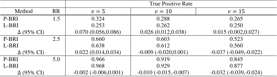
The TPRs for RV associations declared at a marginal BF threshold of BF ≥ 10 are presented in Table I. Overall, we observed higher TPR as well as FPRs for L-BRI relative to P-BRI, indicating marginal BFs to be larger in general
for the L-BRI approach and rendering performance comparisons difficult. When evaluating TPRs at a fixed FPR of
0.01 (Table II), we noted comparable performance. We additionally observed reduced TPR at fixed RR effect sizes
as the proportion of causal variants increased, regardless of method. This is likely due to the fact that models
encompassing a larger number of causal variants are less likely under the default prior distribution on the model
space 𝓜𝓜. In general, performance was comparable between the two approaches, with P-BRI tending to perform better under conditions of lower effect size and smaller proportion of causal variants and L-BRI under large effect
sizes and higher causal variant proportion.
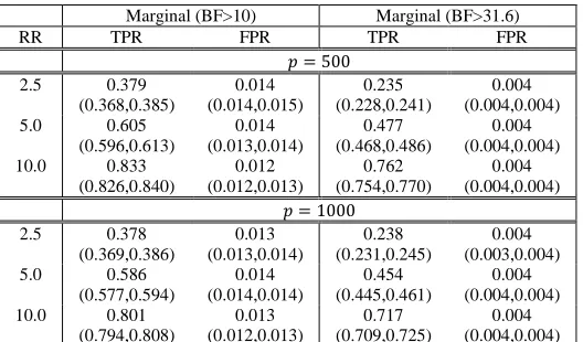
Marginal TPR and FPR results at BF thresholds of 10 and 31.6 for the high RV dimensionality simulations
are presented in Table III. We observed similar patterns of performance with respect to underlying RR and causal
variant proportions as observed in the low RV count simulations, with higher global TPRs for 𝑝𝑝= 500 relative to 𝑝𝑝= 1000 for a fixed causal variant effect size. Marginal RV detection evaluated by TPR and FPR was comparable across differing total number of evaluated variants at a fixed BF threshold, with increasing TPR at higher effect sizes
with the FPR remaining relatively fixed.
The above simulation results do not take into account the likely high degree of multiple testing that would
likely occur prior to post-hoc evaluation, as the simulations only consider the case where true causal variation is
13
controlled at the first stage of testing. To evaluate the behavior of P-BRI under false positive testing results, we
conducted an additional 500 simulations for each of the high variant dimensionality conditions where none of the
simulated variants were associated with case/control status. At a BF threshold of 10, variant-level false positive
rates were commensurate with those reported in Table III (0.012 for 𝑝𝑝 = 500; 0.013 for 𝑝𝑝 = 1000). Data Application
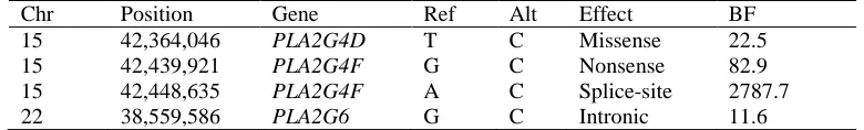
The marginal BFs for the 438 RVs analyzed in the PC risk analysis are presented in Figure 1. A total of four
variants in three separate genes corresponded to a BF >10 (Table IV), including a splice-site variant in gene
PLA2G4F (hg19 chr15:42448635A→T) with a corresponding marginal BF of 2787.7 and PIP of 0.815, occurring in 19 cases but only one control. Both PLA2G4D and PLA2G4F encode proteins thatselectively hydrolyze
glycerophospholipids, and dysregulation of lipid metabolism has been noted in many cancers[Huang and Freter
2015].
To evaluate the MCMC mixing for the data application, we computed the model mutation rate as the
proportion of posterior samples that resulted in model state transitions (77.5%). Computational runtime for the full
30,000 iterations was approximately 20 minutes. Similar application of L-BRI resulted in only 188 accepted model
transitions (mutation rate = 1.25%) for the same number of iterations. After 100,000 iterations (~1 hour runtime) for
two independent runs with a 50,000 burn-in, examination of the marginal BF output from L-BRI still indicated lack
of convergence.
DISCUSSION
In this paper, we have presented a regression-based Bayesian variable selection strategy for post-hoc
analysis of aggregative RV associations in disease risk via a reformulation of the BRI method for case-control RV
association analysis. By modeling the probability of affected status using a probit link function, in contrast to a
logistic regression approach, we have demonstrated the method to be feasible for high dimensional applications. We
have also proposed a component-wise MH algorithm for updating the variable inclusion vector 𝜸𝜸, which results in rapid exploration of the model space. Our simulation results comparing L-BRI and P-BRI for moderate RV counts
indicate that their ability to detect causal RVs is comparable for a variety of conditions, while P-BRI was also
capable of detecting causal variation under very high RV dimensionality. This renders P-BRI a powerful method for
dense post-hoc RV association analyses, as evidenced by both our large-scale simulations and our PC risk analysis
14
associations previously detected by pathway-based analyses may be driven by variants within three phospholipase
genes and additional targeted sequencing of these genes may be warranted in future research.
From a computational perspective, our probit approach benefits from a multi-step MH algorithm for
updating variable inclusion vector 𝜸𝜸. Execution runtimes for P-BRI in our simulation study under conditions where 𝑝𝑝= 50 and 𝑁𝑁= 1000 averaged 6.2 minutes, while runtimes for our larger simulations where 𝑝𝑝= 1000 and 𝑁𝑁= 1000 at 30,000 iterations were approximately 75 minutes on average. The latter analyses were not feasible for L-BRI in our simulations due to the high model space dimensionality and single-step updating of 𝜸𝜸. These timings are based upon working code written in the R statistical language and executed on a modern workstation equipped
with a Quad-Core AMD Opteron™ Processor and 16 Gb of RAM. We anticipate that computational burden for the
P-BRI method may be further reduced substantially with alternative BVS methods, such as objective Bayes model
selection [Leon-Novelo, et al. 2012] and particle stochastic search [Shi and Dunson 2011] approaches, as well as
implementation of parts of the current MCMC algorithm in more computationally efficient computer languages such
as C++.
A simplifying assumption of risk index methods in general is that each included RV contributes an equal
effect to the RV burden, or rather that it models the mean effect of the selected RVs. While this assumption permits
efficient sampling, it may not accurately reflect the effects of the individual RV associations. It is possible to utilize
existing structural definitions, such as genes or exons, as a grouping mechanism and assign separate burden-based
parameters, although careful consideration is necessary to avoid singular design matrices if the number of included
elements exceeds the sample size. If protective RV’s are present, they would not be appropriately modeled by our
approach. However, the P-BRI method could be simply modified by increasing the support of 𝜸𝜸 to include negative indicators, as in the MixBRI approach by Quintana et al. [Quintana, et al. 2011].
Although the P-BRI method permits efficient exploration of high-dimensional model spaces, alternative
MH algorithms for sampling from the model space 𝓜𝓜may be useful in extreme scenarios where the RV
dimensionality renders the component-wise MH algorithm computationally infeasible. One approach is to consider
15
with 𝑝𝑝 ≥ 10,000, although further work is necessary to formally develop these methods. Adaptive algorithms designed for high-dimensional sampling in GWAS may also be of utility[Peltola, et al. 2012].
There are a variety of promising extensions from our development of the P-BRI method for post-hoc RV
analysis. An added benefit of this work is that application to quantitative traits is trivial, since the algorithms are
already in place through the latent variable 𝒀𝒀�, although variational Bayesian methods have previously demonstrated high computational efficiency in this area[Logsdon, et al. 2014]. We could also extend the regression procedure to
include common variants in the model selection for a comprehensive association analysis, as well as easily adopt the
integrative variable selection procedures in Quintana et al. [Quintana and Conti 2013] for informed model selection
based upon existing variant annotation. Finally, we are actively evaluating methods to estimate global null model
posterior probabilities using sampling procedures implemented by Liang et al.[Liang and Xiong 2013] for
association inference, as well as integrating P-BRI methods with curated pathway databases to facilitate
genome-wide exploratory rare variant gene-set analysis.
ACKNOWLEDGEMENTS
This research was supported by the US Public Health Service, National Institutes of Health (NIH), contract Grant
Number GM065450 (DJS) and
National Cancer Institute, Grant number U01 CA 89600 (SNT). There are no
conflicts of interest to declare.
REFERENCES
Albert JH, Chib S. 1993. Bayesian-Analysis of Binary and Polychotomous Response Data. Journal of the
American Statistical Association 88(422):669-679.
Bansal V, Libiger O, Torkamani A, Schork NJ. 2010. Statistical analysis strategies for association studies
involving rare variants. Nature reviews. Genetics 11(11):773-85.
Baragatti M. 2011. Bayesian Variable Selection for Probit Mixed Models Applied to Gene Selection.
Bayesian Analysis 6(2):209-229.
Cirulli ET, Goldstein DB. 2010. Uncovering the roles of rare variants in common disease through
whole-genome sequencing. Nature Reviews Genetics 11(6):415-425.
DePristo MA, Banks E, Poplin R, Garimella KV, Maguire JR, Hartl C, Philippakis AA, del Angel G, Rivas MA,
Hanna M and others. 2011. A framework for variation discovery and genotyping using
next-generation DNA sequencing data. Nature genetics 43(5):491-8.
Dering C, Hemmelmann C, Pugh E, Ziegler A. 2011. Statistical analysis of rare sequence variants: an
overview of collapsing methods. Genetic epidemiology 35:S12-S17.
16
Hastings WK. 1970. Monte Carlo sampling methods using Markov chains and their applications.
Biometrika 57(1):97-109.
Huang C, Freter C. 2015. Lipid metabolism, apoptosis and cancer therapy. International journal of
molecular sciences 16(1):924-49.
Jeffreys H. 1961. Theory of probability. Oxford,: Clarendon Press.
Johnson AA, Jones GL, Neath RC. 2013. Component-Wise Markov Chain Monte Carlo: Uniform and
Geometric Ergodicity under Mixing and Composition. Statistical Science 28(3):360-375.
Joshi-Tope G, Gillespie M, Vastrik I, D'Eustachio P, Schmidt E, de Bono B, Jassal B, Gopinath GR, Wu GR,
Matthews L and others. 2005. Reactome: a knowledgebase of biological pathways. Nucleic acids
research 33(Database issue):D428-32.
Kanehisa M. 2002. The KEGG database. Novartis Foundation symposium 247:91-101; discussion 101-3,
119-28, 244-52.
Kang G, Bi W, Zhao Y, Zhang JF, Yang JJ, Xu H, Loh ML, Hunger SP, Relling MV, Pounds S and others. 2014.
A new system identification approach to identify genetic variants in sequencing studies for a
binary phenotype. Human heredity 78(2):104-16.
Lee KE, Sha NJ, Dougherty ER, Vannucci M, Mallick BK. 2003. Gene selection: a Bayesian variable
selection approach. Bioinformatics 19(1):90-97.
Lee KJ, Jones GL, Caffo BS, Bassett SS. 2014. Spatial Bayesian Variable Selection Models on Functional
Magnetic Resonance Imaging Time-Series Data. Bayesian Analysis 9(3):699-732.
Lee S, Emond MJ, Bamshad MJ, Barnes KC, Rieder MJ, Nickerson DA, Christiani DC, Wurfel MM, Lin X.
2012. Optimal unified approach for rare-variant association testing with application to
small-sample case-control whole-exome sequencing studies. American journal of human genetics
91(2):224-37.
Leon-Novelo L, Moreno E, Casella G. 2012. Objective Bayes model selection in probit models. Statistics in
medicine 31(4):353-365.
Li B, Leal SM. 2008. Methods for detecting associations with rare variants for common diseases:
application to analysis of sequence data. American journal of human genetics 83(3):311-21.
Liang FM, Xiong MM. 2013. Bayesian Detection of Causal Rare Variants under Posterior Consistency.
PloS one 8(7).
Liu JS. 1994. The Collapsed Gibbs Sampler in Bayesian Computations with Applications to a
Gene-Regulation Problem. Journal of the American Statistical Association 89(427):958-966.
Liu JS. 1996. Peskun's theorem and a modified discrete-state Gibbs sampler. Biometrika 83(3):681-682.
Logsdon BA, Dai JY, Auer PL, Johnsen JM, Ganesh SK, Smith NL, Wilson JG, Tracy RP, Lange LA, Jiao S and
others. 2014. A variational Bayes discrete mixture test for rare variant association. Genetic
epidemiology 38(1):21-30.
McKenna A, Hanna M, Banks E, Sivachenko A, Cibulskis K, Kernytsky A, Garimella K, Altshuler D, Gabriel
S, Daly M and others. 2010. The Genome Analysis Toolkit: a MapReduce framework for
analyzing next-generation DNA sequencing data. Genome research 20(9):1297-303.
Neale BM, Rivas MA, Voight BF, Altshuler D, Devlin B, Orho-Melander M, Kathiresan S, Purcell SM,
Roeder K, Daly MJ. 2011. Testing for an unusual distribution of rare variants. Plos Genetics
7(3):e1001322.
Nelson MR, Wegmann D, Ehm MG, Kessner D, St Jean P, Verzilli C, Shen J, Tang Z, Bacanu SA, Fraser D
and others. 2012. An abundance of rare functional variants in 202 drug target genes sequenced
in 14,002 people. Science 337(6090):100-4.
17
Peltola T, Marttinen P, Vehtari A. 2012. Finite adaptation and multistep moves in the
metropolis-hastings algorithm for variable selection in genome-wide association analysis. PloS one
7(11):e49445.
Pritchard JK. 2001. Are rare variants responsible for susceptibility to complex diseases? American journal
of human genetics 69(1):124-37.
Quintana MA, Berstein JL, Thomas DC, Conti DV. 2011. Incorporating model uncertainty in detecting rare
variants: the Bayesian risk index. Genetic epidemiology 35(7):638-49.
Quintana MA, Conti DV. 2013. Integrative variable selection via Bayesian model uncertainty. Statistics in
medicine.
Shi MH, Dunson DB. 2011. Bayesian variable selection via particle stochastic search. Statistics &
Probability Letters 81(2):283-291.
Tanner MA, Wing HW. 1987. The Calculation of Posterior Distributions by Data Augmentation -
Rejoinder. Journal of the American Statistical Association 82(398):548-550.
Thomson PA, Parla JS, McRae AF, Kramer M, Ramakrishnan K, Yao J, Soares DC, McCarthy S, Morris SW,
Cardone L and others. 2013. 708 Common and 2010 rare DISC1 locus variants identified in 1542
subjects: analysis for association with psychiatric disorder and cognitive traits. Molecular
psychiatry.
Van der Auwera GA, Carneiro MO, Hartl C, Poplin R, Del Angel G, Levy-Moonshine A, Jordan T, Shakir K,
Roazen D, Thibault J and others. 2013. From FastQ data to high confidence variant calls: the
Genome Analysis Toolkit best practices pipeline. Current protocols in bioinformatics / editoral
board, Andreas D. Baxevanis ... [et al.] 11(1110):11 10 1-11 10 33.
Wilson MA, Iversen ES, Clyde MA, Schmidler SC, Schildkraut JM. 2010. Bayesian Model Search and
Multilevel Inference for Snp Association Studies. Annals of Applied Statistics 4(3):1342-1364.
Wu G, Zhi D. 2013. Pathway-based approaches for sequencing-based genome-wide association studies.
Genetic epidemiology 37(5):478-94.
Wu MC, Lee S, Cai TX, Li Y, Boehnke M, Lin XH. 2011. Rare-Variant Association Testing for Sequencing
Data with the Sequence Kernel Association Test. American journal of human genetics
89(1):82-93.
Yang AJ, Song XY. 2010. Bayesian variable selection for disease classification using gene expression data.
Bioinformatics 26(2):215-22.
Zellner A. 1983. Applications of Bayesian-Analysis in Econometrics. Statistician 32(1-2):23-34.
Zhou H, Sehl ME, Sinsheimer JS, Lange K. 2010. Association screening of common and rare genetic
variants by penalized regression. Bioinformatics 26(19):2375-82.
SUPPLEMENTARY METHODSDefining component-wise MH algorithm
Note that
𝑖𝑖�𝒀𝒀��𝜸𝜸,𝜷𝜷�=∫ 𝑖𝑖�𝒀𝒀��𝜸𝜸,−∞∞ 𝜷𝜷,𝛽𝛽𝛾𝛾�𝑖𝑖�𝛽𝛽𝛾𝛾�𝑑𝑑𝛽𝛽𝛾𝛾 ∝ ∫−∞∞ exp�−21�𝒀𝒀� − 𝑿𝑿𝜷𝜷 − 𝒁𝒁𝜸𝜸𝛽𝛽𝛾𝛾�′�𝒀𝒀� − 𝑿𝑿𝜷𝜷 − 𝒁𝒁𝜸𝜸𝛽𝛽𝛾𝛾�� 𝑖𝑖�𝛽𝛽𝛾𝛾�𝑑𝑑𝛽𝛽𝛾𝛾.
Note expansion of the term �𝒀𝒀� − 𝑿𝑿𝜷𝜷 − 𝒁𝒁𝜸𝜸𝛽𝛽𝛾𝛾�′𝑰𝑰𝑵𝑵−𝟏𝟏�𝒀𝒀� − 𝑿𝑿𝜷𝜷 − 𝒁𝒁𝜸𝜸𝛽𝛽𝛾𝛾� yields
18
From the above, we can rewrite 𝑖𝑖�𝒀𝒀��𝜸𝜸,𝜷𝜷� as proportional to
exp�−12�𝒀𝒀� − 𝑿𝑿𝜷𝜷�′�𝒀𝒀� − 𝑿𝑿𝜷𝜷��×∫∞ exp�−21�𝛽𝛽𝛾𝛾2𝒁𝒁𝜸𝜸′𝒁𝒁𝜸𝜸−2𝛽𝛽𝛾𝛾��𝒀𝒀� − 𝑿𝑿𝜷𝜷�′𝒁𝒁𝜸𝜸��� 𝑖𝑖�𝛽𝛽𝛾𝛾�𝑑𝑑𝛽𝛽𝛾𝛾
−∞ .
Given that the prior distribution on 𝛽𝛽𝛾𝛾 is 𝑖𝑖�𝛽𝛽𝛾𝛾�=�2𝜋𝜋𝜎𝜎1 𝛽𝛽exp�−𝛽𝛽𝛾𝛾
2
2𝜎𝜎𝛽𝛽2�, it follows that
∫∞ exp�−12�𝛽𝛽𝛾𝛾2𝒁𝒁𝜸𝜸′𝒁𝒁𝜸𝜸 −2𝛽𝛽𝛾𝛾��𝒀𝒀� − 𝑿𝑿𝜷𝜷�′𝒁𝒁𝜸𝜸��� 𝑖𝑖�𝛽𝛽𝛾𝛾�𝑑𝑑𝛽𝛽𝛾𝛾
−∞ ∝ ∫ exp�−
1
2�𝛽𝛽𝛾𝛾2𝒁𝒁𝜸𝜸′𝒁𝒁𝜸𝜸−2𝛽𝛽𝛾𝛾��𝒀𝒀� − 𝑿𝑿𝜷𝜷� ′
𝒁𝒁𝜸𝜸�+ ∞
−∞
1
𝜎𝜎𝛽𝛽2𝛽𝛽𝛾𝛾2�� 𝑑𝑑𝛽𝛽𝛾𝛾.
We can complete the square in the exponential term, such that
𝛽𝛽𝛾𝛾2𝒁𝒁𝜸𝜸′𝒁𝒁𝜸𝜸−2𝛽𝛽𝛾𝛾��𝒀𝒀� − 𝑿𝑿𝜷𝜷�′𝒁𝒁𝜸𝜸�+𝛽𝛽𝛾𝛾2=�𝒁𝒁𝜸𝜸′𝒁𝒁𝜸𝜸+𝜎𝜎
𝛽𝛽−2� �𝛽𝛽𝛾𝛾− �𝒀𝒀�−𝑿𝑿𝜷𝜷�
′𝒁𝒁 𝜸𝜸
�𝒁𝒁𝜸𝜸′𝒁𝒁𝜸𝜸+𝜎𝜎𝛽𝛽−2�� − �𝒁𝒁𝜸𝜸
′𝒁𝒁𝜸𝜸+𝜎𝜎
𝛽𝛽−2� ��𝒀𝒀�−𝑿𝑿𝜷𝜷�
′𝒁𝒁 𝜸𝜸
�𝒁𝒁𝜸𝜸′𝒁𝒁𝜸𝜸+𝜎𝜎𝛽𝛽−2��
2
.
Given the presence of the Gaussian kernel, it follows that
∫ exp�−12�𝛽𝛽𝛾𝛾2𝒁𝒁𝜸𝜸′𝒁𝒁𝜸𝜸−2𝛽𝛽𝛾𝛾��𝒀𝒀� − 𝑿𝑿𝜷𝜷�′𝒁𝒁𝜸𝜸�+𝛽𝛽𝛾𝛾2�� 𝑑𝑑𝛽𝛽 𝛾𝛾 ∞
−∞ ∝exp�
1 2
��𝒀𝒀�−𝑿𝑿𝜷𝜷�′𝒁𝒁𝜸𝜸� 𝟐𝟐
�𝒁𝒁𝜸𝜸′𝒁𝒁𝜸𝜸+𝜎𝜎𝛽𝛽−2� �. Note the following
��𝒀𝒀�−𝑿𝑿𝜷𝜷�′𝒁𝒁𝜸𝜸�𝟐𝟐
�𝒁𝒁𝜸𝜸′𝒁𝒁𝜸𝜸+𝜎𝜎𝛽𝛽−2� =
1
𝒁𝒁𝜸𝜸′𝒁𝒁𝜸𝜸+𝜎𝜎𝛽𝛽−2�𝒀𝒀� − 𝑿𝑿𝜷𝜷�
′
𝒁𝒁𝜸𝜸𝒁𝒁𝜸𝜸′ (𝒀𝒀� − 𝑿𝑿𝜷𝜷).
It then follows that
𝑖𝑖�𝒀𝒀��𝜸𝜸,𝜷𝜷� ∝exp�−12��𝒀𝒀� − 𝑿𝑿𝜷𝜷�′�𝑰𝑰𝑵𝑵− 𝒁𝒁𝜸𝜸𝒁𝒁𝜸𝜸′
�𝒁𝒁𝜸𝜸′𝒁𝒁𝜸𝜸+𝜎𝜎𝛽𝛽−2�� �𝒀𝒀� − 𝑿𝑿𝜷𝜷���.
Then,
𝑖𝑖�𝜸𝜸�𝒀𝒀�,𝜷𝜷� ∝ 𝑖𝑖�𝒀𝒀��𝜸𝜸,𝜷𝜷�𝑖𝑖(𝜸𝜸)∝exp�−12��𝒀𝒀� − 𝑿𝑿𝜷𝜷�′�𝑰𝑰𝑵𝑵− 𝒁𝒁𝜸𝜸𝒁𝒁𝜸𝜸 ′
�𝒁𝒁𝜸𝜸′𝒁𝒁𝜸𝜸+𝜎𝜎
𝛽𝛽−2�� �𝒀𝒀� − 𝑿𝑿𝜷𝜷���×� 𝜋𝜋𝑖𝑖 𝛾𝛾𝑗𝑗�1− 𝜋𝜋
𝑖𝑖�1−𝛾𝛾𝑗𝑗 𝑝𝑝
𝑖𝑖=1
.
19
𝜌𝜌�𝜸𝜸(𝑡𝑡),𝜸𝜸(⋆)� = min ⎝ ⎜ ⎜ ⎜ ⎜⎛𝑒𝑒𝑒𝑒𝑝𝑝 �12��(𝒁𝒁𝜸𝜸(⋆))′𝒁𝒁𝜸𝜸1(⋆)+𝜎𝜎
𝛽𝛽−2��𝒀𝒀� − 𝑿𝑿𝜷𝜷� ′
𝒁𝒁𝜸𝜸(⋆)�𝒁𝒁𝜸𝜸(⋆)�′�𝒀𝒀� − 𝑿𝑿𝜷𝜷��� ∏ 𝜋𝜋 𝑖𝑖
𝛾𝛾𝑗𝑗(⋆)
�1− 𝜋𝜋𝑖𝑖�1−𝛾𝛾𝑗𝑗(⋆)
𝑟𝑟 𝑖𝑖=1
𝑒𝑒𝑒𝑒𝑝𝑝 �12��(𝒁𝒁𝜸𝜸(𝑡𝑡))′𝒁𝒁𝜸𝜸1(𝑡𝑡)+𝜎𝜎
𝛽𝛽−2��𝒀𝒀� − 𝑿𝑿𝜷𝜷� ′
𝒁𝒁𝜸𝜸(𝑡𝑡)(𝒁𝒁𝜸𝜸(𝑡𝑡))′�𝒀𝒀� − 𝑿𝑿𝜷𝜷��� ∏ 𝜋𝜋 𝑖𝑖
𝛾𝛾𝑗𝑗(𝑡𝑡)
�1− 𝜋𝜋𝑖𝑖�1−𝛾𝛾𝑗𝑗(𝑡𝑡)
𝑟𝑟 𝑖𝑖=1 , 1 ⎠ ⎟ ⎟ ⎟ ⎟ ⎞
𝜌𝜌�𝜸𝜸(𝑡𝑡),𝜸𝜸(⋆)�= min�exp�1
2�𝒀𝒀� − 𝑿𝑿𝜷𝜷� ′
� 𝒁𝒁𝜸𝜸(⋆)�𝒁𝒁𝜸𝜸(⋆)� ′
𝜎𝜎𝛽𝛽−2+ (𝒁𝒁𝜸𝜸(⋆))′(𝒁𝒁𝜸𝜸(⋆))−
𝒁𝒁𝜸𝜸(𝑡𝑡)�𝒁𝒁𝜸𝜸(𝑡𝑡)�′
𝜎𝜎𝛽𝛽−2+ (𝒁𝒁𝜸𝜸(𝑡𝑡))′(𝒁𝒁𝜸𝜸(𝑡𝑡))� �𝒀𝒀�
− 𝑿𝑿𝜷𝜷�� � �1− 𝜋𝜋𝜋𝜋𝑖𝑖 𝑖𝑖�
𝛾𝛾𝑗𝑗(⋆)−𝛾𝛾𝑗𝑗(𝑡𝑡) 𝑟𝑟
𝑖𝑖=1
, 1�
For component-wise updating of 𝜸𝜸, note that
𝑖𝑖�𝛾𝛾𝑖𝑖�𝒀𝒀�,𝜷𝜷,𝜸𝜸(−𝒋𝒋)� ∝ 𝑖𝑖(𝒀𝒀�|𝜸𝜸,𝜷𝜷) ×� 𝜋𝜋𝑗𝑗
1−𝜋𝜋𝑗𝑗�
𝛾𝛾𝑗𝑗(⋆)−𝛾𝛾𝑗𝑗(𝑡𝑡)
,
where 𝜸𝜸(−𝒋𝒋) indicates the vector of values in𝜸𝜸 other than 𝛾𝛾𝑖𝑖. Then𝜸𝜸(⋆) differs from 𝜸𝜸(𝒕𝒕) at the 𝑗𝑗𝑡𝑡ℎ element, such that 𝛾𝛾𝑖𝑖(⋆)= 1 if 𝛾𝛾𝑖𝑖(𝑡𝑡)= 0 or 𝛾𝛾𝑖𝑖(⋆)= 0 if 𝛾𝛾𝑖𝑖(𝑡𝑡)= 1. We can reparameterize the acceptance probability with respect to 𝒁𝒁𝜸𝜸 =𝒁𝒁𝜸𝜸, such that
𝒁𝒁𝜸𝜸(⋆)=𝒁𝒁𝜸𝜸(𝒕𝒕)±𝒁𝒁𝒋𝒋,
where 𝒁𝒁𝒋𝒋 is the 𝑗𝑗𝑡𝑡ℎ column of 𝒁𝒁 and the sign of the operation (+ or -) is dictated by the current state of 𝛾𝛾𝑖𝑖. Simplify notation by 𝒀𝒀�𝒓𝒓𝒓𝒓𝒓𝒓=𝒀𝒀� − 𝑿𝑿𝜷𝜷, and we write 𝜌𝜌�𝛾𝛾𝑖𝑖(𝑡𝑡),𝛾𝛾𝑖𝑖(⋆)� as
min�exp�12𝒀𝒀�𝑟𝑟𝑟𝑟𝑟𝑟′ � �𝒁𝒁𝜸𝜸(𝒕𝒕)±𝒁𝒁𝒋𝒋��𝒁𝒁𝜸𝜸(𝒕𝒕)±𝒁𝒁𝒋𝒋�′
𝜎𝜎𝛽𝛽−2+�𝒁𝒁𝜸𝜸(𝒕𝒕)±𝒁𝒁𝒋𝒋�′�𝒁𝒁𝜸𝜸(𝒕𝒕)±𝒁𝒁𝒋𝒋�−
�𝒁𝒁𝜸𝜸(𝒕𝒕)��𝒁𝒁𝜸𝜸(𝒕𝒕)�′
𝜎𝜎𝛽𝛽−2+�𝒁𝒁𝜸𝜸(𝒕𝒕)�′�𝒁𝒁𝜸𝜸(𝒕𝒕)�� 𝒀𝒀�𝑟𝑟𝑟𝑟𝑟𝑟� � 𝜋𝜋𝑗𝑗
1−𝜋𝜋𝑗𝑗�
𝛾𝛾𝑗𝑗(⋆)−𝛾𝛾𝑗𝑗(𝑡𝑡) , 1�.
Define 𝑎𝑎(⋆)= 1
𝜎𝜎𝛽𝛽−2+�𝒁𝒁𝜸𝜸(𝒕𝒕)±𝒁𝒁𝒋𝒋� ′
�𝒁𝒁𝜸𝜸(𝒕𝒕)±𝒁𝒁𝒋𝒋�
and 𝑎𝑎(𝑡𝑡) = 1
𝜎𝜎𝛽𝛽−2+�𝒁𝒁𝜸𝜸(𝒕𝒕)�′�𝒁𝒁𝜸𝜸(𝒕𝒕)�. It then follows that 𝜌𝜌�𝛾𝛾𝑖𝑖 (𝑡𝑡),𝛾𝛾
𝑖𝑖(⋆)� simplifies to
min�exp�12 ��𝑎𝑎(⋆)− 𝑎𝑎(𝑡𝑡)��𝒀𝒀� 𝑟𝑟𝑟𝑟𝑟𝑟 ′ 𝒁𝒁
𝜸𝜸
(𝒕𝒕)�2± 2𝑎𝑎(⋆)�𝒀𝒀� 𝑟𝑟𝑟𝑟𝑟𝑟 ′ 𝒁𝒁 𝜸𝜸 (𝒕𝒕)��𝒀𝒀� 𝑟𝑟𝑟𝑟𝑟𝑟 ′ 𝒁𝒁
𝒋𝒋�+𝑎𝑎(⋆)�𝒀𝒀�𝑟𝑟𝑟𝑟𝑟𝑟′ 𝒁𝒁𝒋𝒋�2�� �1−𝜋𝜋𝜋𝜋𝑗𝑗𝑗𝑗� 𝛾𝛾𝑗𝑗(⋆)−𝛾𝛾𝑗𝑗(𝑡𝑡)
, 1�.
Values of 𝒀𝒀�𝑟𝑟𝑟𝑟𝑟𝑟′ 𝒁𝒁𝒋𝒋 ∀ 𝑗𝑗 can be calculated in advance of the MH step, and 𝒀𝒀�𝑟𝑟𝑟𝑟𝑟𝑟′ 𝒁𝒁𝜸𝜸(𝒕𝒕)can be easily updated in the sub-steps if the proposal is accepted by updating to 𝒀𝒀�𝑟𝑟𝑟𝑟𝑟𝑟′ 𝒁𝒁𝜸𝜸(𝒕𝒕)±𝒀𝒀�𝑟𝑟𝑟𝑟𝑟𝑟′ 𝒁𝒁𝒋𝒋.
20
Pathway-based testing was conducted in R using the package SKAT using pathway definitions from KEGG and Reactome. These analyses were conducted on independent samples by selecting a random individual from each of the sequenced pedigrees. The application of the probit BVS method was applied to the same set of samples.
For analysis, variant sets were formed by aggregating variants within genes and then genes within
21
TABLES𝑣𝑣= 5 𝑣𝑣= 10 𝑣𝑣= 15
Method RR TPR FPR TPR FPR TPR FPR
P-BRI 1.5 0.341
(0.323,0.360) 0.012 (0.011,0.014) 0.331 (0.317,0.344) 0.014 (0.013,0.016) 0.313 (0.303,0.324) 0.015 (0.013,0016)
L-BRI 0.314
(0.295,0.333) 0.017 (0.015,0.019) 0.405 (0.391,0.417) 0.030 (0.028,0.033) 0.434 (0.423,0.445) 0.039 (0.036,0.042)
P-BRI 2.5 0.694
(0.677,0.713) 0.014 (0.012,0.015) 0.643 (0.630,0.656) 0.014 (0.013,0.016) 0.569 (0.558,0.581) 0.014 (0.012,0016)
L-BRI 0.761
(0.746,0.779) 0.035 (0.033,0.038) 0.806 (0.796,0.817) 0.058 (0.055,0.061) 0.784 (0.774,0.793) 0.070 (0.067,0.074)
P-BRI 5.0 0.972
(0.966,0.978) 0.013 (0.012,0.015) 0.929 (0.923,0,936) 0.014 (0.013,0.016) 0.867 (0.859,0.875) 0.014 (0.013,0016)
L-BRI 0.986
(0.981,0.990) 0.039 (0.036,0.041) 0.978 (0.974,0.982) 0.061 (0.058,0.064) 0.965 (0.961,0.969) 0.090 (0.086,0.095)
Table I: Simulation results for empirical TPRs and FPRs and corresponding bootstrapped 95% confidence intervals for causal RV detection across simulation replications with fixed marginal BF threshold set to 10 (“strong”
22
True Positive Rate
Method RR 𝑣𝑣= 5 𝑣𝑣= 10 𝑣𝑣= 15
P-BRI 1.5 0.324 0.288 0.265
L-BRI 0.253 0.262 0.250
Δ (95% CI) 0.070 (0.056,0.086) 0.026 (0.012,0.038) 0.015 (0.002,0.027)
P-BRI 2.5 0.660 0.603 0.523
L-BRI 0.638 0.612 0.560
Δ (95% CI) 0.022 (0.014,0.034) -0.009 (-0.020,0.001) -0.037 (-0.049,-0.022)
P-BRI 5.0 0.966 0.919 0.845
L-BRI 0.968 0.929 0.877
Δ (95% CI) -0.002 (-0.006,0.001) -0.010 (-0.015,-0.007) -0.032 (-0.039,-0.024) Table II: Simulation results for empirical TPRs for causal RV detection across simulation replications at a fixed
23
Marginal (BF>10) Marginal (BF>31.6)
RR TPR FPR TPR FPR
𝑝𝑝= 500
2.5 0.379
(0.368,0.385) 0.014 (0.014,0.015) 0.235 (0.228,0.241) 0.004 (0.004,0.004)
5.0 0.605
(0.596,0.613) 0.014 (0.013,0.014) 0.477 (0.468,0.486) 0.004 (0.004,0.004)
10.0 0.833
(0.826,0.840) 0.012 (0.012,0.013) 0.762 (0.754,0.770) 0.004 (0.004,0.004) 𝑝𝑝= 1000
2.5 0.378
(0.369,0.386) 0.013 (0.013,0.014) 0.238 (0.231,0.245) 0.004 (0.003,0.004)
5.0 0.586
(0.577,0.594) 0.014 (0.014,0.014) 0.454 (0.445,0.461) 0.004 (0.004,0.004)
10.0 0.801
(0.794,0.808) 0.013 (0.012,0.013) 0.717 (0.709,0.725) 0.004 (0.004,0.004)
24
Chr Position Gene Ref Alt Effect BF
15 42,364,046 PLA2G4D T C Missense 22.5
15 42,439,921 PLA2G4F G C Nonsense 82.9
15 42,448,635 PLA2G4F A C Splice-site 2787.7
22 38,559,586 PLA2G6 G C Intronic 11.6
25
FIGURE DESCRIPTIONS