Numerical simulation of ﬂoating bodies in extreme free surface waves

(1)

www.nat-hazards-earth-syst-sci.net/11/519/2011/ doi:10.5194/nhess-11-519-2011

Natural Hazards

and Earth

System Sciences

Numerical simulation of floating bodies in extreme free

surface waves

Z. Z. Hu, D. M. Causon, C. G. Mingham, and L. Qian

Centre for Mathematical Modelling and Flow analysis, School of Computing, Mathematics and Digital Technology, The Manchester Metropolitan University, Manchester, M1 5GD, UK

Received: 20 July 2010 – Revised: 12 January 2011 – Accepted: 12 January 2011 – Published: 16 February 2011

Abstract. In this paper, we use the in-house Computational

Fluid Dynamics (CFD) flow code AMAZON-SC as a numerical wave tank (NWT) to study wave loading on a wave energy converter (WEC) device in heave motion. This is a surface-capturing method for two fluid flows that treats the free surface as contact surface in the density field that is captured automatically without special provision. A time-accurate artificial compressibility method and high resolution Godunov-type scheme are employed in both fluid regions (air/water). The Cartesian cut cell method can provide a boundary-fitted mesh for a complex geometry with no requirement to re-mesh globally or even locally for moving geometry, requiring only changes to cut cell data at the body contour. Extreme wave boundary conditions are prescribed in an empty NWT and compared with physical experiments prior to calculations of extreme waves acting on a floating Bobber-type device. The validation work also includes the wave force on a fixed cylinder compared with theoretical and experimental data under regular waves. Results include free surface elevations, vertical displacement of the float, induced vertical velocity and heave force for a typical Bobber geometry with a hemispherical base under extreme wave conditions.

1 Introduction

In this paper, we describe developments of the AMAZON-SC 3D numerical wave tank (NWT) to study extreme wave loading of a floating structure (in Heave motion). The extreme wave formulation prescribed as an inlet condition is due to Dalzell (1999) and Ning et al. (2009) is based on a first or second-order Stokes focused wave.

Correspondence to: Z. Z. Hu

([email protected])

The AMAZON-SC 3D code (see e.g. Hu et al., 2009) uses a cell centred finite volume method of the Godunov-type for the space discretization of the Euler and Navier Stokes equations. The computational domain includes both air and water regions with the air/water boundary captured as a discontinuity in the density field thereby admitting the break up and recombination of the free surface. Temporal discretisation uses the artificial compressibility method and a dual time stepping strategy to maintain a divergence free velocity field. Cartesian cut cells are used to provide a fully boundary-fitted gridding capability on a regular background Cartesian grid. Solid objects are cut out of the background mesh leaving a set of irregularly shaped cells fitted to the boundary. The advantages of the cut cell approach have been outlined previously by Causon et al. (2000, 2001) including its flexibility for dealing with complex geometries whether stationary or in relative motion. The field grid does not need to be recomputed globally or even locally for moving body cases; all that is necessary is to update the local cut cell data at the body contour for as long as the motion continues. The handing of numerical wave paddles and device motion in the AMAZON-SC NWT is therefore straightforward and efficient.

Firstly, extreme design wave conditions are generated in an empty NWT and compared with laboratory measurements as a precursor to calculations to investigate the survivability of the Bobber device operating in a challenging wave climate. Secondly, a fixed submergence horizontal cylinder has been validated in regular waves. Finally, a floating Bobber has been simulated under extreme wave conditions.

2 The Cartesian cut cell mesh

(2)

520 Z. Z. Hu et al.: Numerical simulation of floating bodies a regular Cartesian mesh. Moving flow boundaries or bodies

in relative motion within the flow domain are accommodated by computing local cell-boundary intersections at the boundaries that are in motion. A detailed description of the principles of the cut cell method including the numerical procedures applied at solid boundaries that are either static or in relative motion have been given previously by the authors (Yang et al., 1997; Causon et al., 2000, 2001; Qian et al., 2003) including extension of the cut cell algorithms to 3-D (Yang et al., 2000; Hu et al., 2009).

3 The flow solver on a cut cell mesh

The Euler equations for a general moving control volume of fluid expressed in a pseudo-compressible form can be written as

∂ ∂t

Z Z

V

Z

Q∂V+

I

S

F ·n∂s=

Z Z

V

Z

B∂V (1)

where Q is the vector of conserved variables within the volumeV,F is the conservative flux through the volume’s bounding surface S, whose outward-pointing unit-normal vector isnand B is a source term of body forces. Q, F andBare given by

Q=

ρ,ρu,ρv,ρw,p β

T

, (2)

F =fInx+gIny+hInz, (3)

B =[0,0,0,−ρg,0]T (4)

where

fI =[ρ (u−ub),ρu(u−ub)+p,ρv (u−ub),ρw(u−ub),u]T,

gI =[ρ (v−vb),ρu(v−vb),ρv (v−vb)+p,ρw(v−vb),v]T,

hI =[ρ (w−wb),ρu(w−wb),ρv (w−wb),ρw(w−wb)+p,w]T, where u, v and w are the flow velocity components and ub, vb and wb are the velocity components of the

(body) boundary S, which are identically zero when the boundary is stationary. ρ is the fluid density, p is the pressure, β is the coefficient of artificial compressibility and g is the gravitational acceleration. The use of a pseudo-compressible form of the describing equations and artificial compressibility parameter β permits the use of efficient modern Riemann-based solution methods developed for compressible flows.

We then discretize Eq. (1) over each cell of the flow domain using a finite volume formulation, which gives

∂Q_{ij k}Vij k

∂t = −

r

X

k=1

Fk1Ak+BVij k= −R Qij k, (5)

whereQij k is the average value of the solution vector Q at cell (i, j, k) stored at the cell centre and Vij k denotes the volume of the cell. Fk is the numerical flux across the bounded facekof the finite volume cell,1Ak is the area of that face andris an integer identifier for each face of the cell (>4 in the case of a 2-D cut cell).

The convective fluxFk in Eq. (5) is then determined by solving a Riemann problem at each cell interface. This involves two stages: first, the left and right state values are reconstructed on the opposite sides of each cell face by projecting the solution data from the stored cell centre values either side of the cell face centre; second, the resulting Riemann problem defined by the left and right state data is solved using an approximate Riemann solver (ARS).

Thus, the required left and right state values corresponding to stored cell centre dataQ(x,y,z)can be found anywhere within the cut cell using

Q(x,y,z)=Qi,j,k+1Qi,j,k×r (6)

whereris the normal distance vector from the cell centre to any specific interface or solid boundary. Qi,j,kis the stored computed cell centre data and1Qij k is the gradient at cell (i,j,k).

Secondly, Roe’s approximate flux Fk is constructed to second order accuracy in each cell. This assumes a 1-D Riemann problem in the direction normal to the cell face and has the form

Fk= 1 2

h

Fk(QR)+Fk(QL)−

˜ A

(QR−QL) i

,

˜ A

=R|3|L (7)

whereQRandQL are the reconstructed data values on the

right and left of facek based on Eq. (6) and _A˜ _{is the flux} Jacobian evaluated using Roe’s average state values Q˜ =

˜

Q(QL,QR). The quantities R andLare the right and left

eigenvectors of A˜. 3 is the diagonal eigenvalue matrix, |3| =diag(λ1,λ2,λ3,λ4,λ5)where the eigenvalues are given

by

λ1,2,3=unx+vny+wnz,λ4,5=0.5 unx+vny+wnz±C (8) whereC=

q

unx+vny+wnz2+4β/ρ.

The Jacobian matrix A can be constructed according to its definition A=∂ (F·n)/∂Q,

A= 

    

0 nx ny nz 0

−u2_n

x−uvny−uwnz2unx+vny+wnz uny unz βnx

−uvnx−v2ny−vwnz vnx unx+2vny+wnz vnz βny

−uwnx−vwny−w2nz wnx wny unx+vny+2wnzβnz

−unx ρ −

vny ρ −

wnz ρ

nx ρ

ny ρ

nz

ρ 0



    

(9)

(3)

The approximate Roe average is obtained at each cell facek by computing

˜

Q=↔ρ ,ρ˜u,˜ ρ˜v,˜ ρ˜w,˜ p/β˜ for the two fluid flows gives

˜

ρ=√ρRρL, u˜=uL

√ ρL+uR

√ ρR/

√ ρL+

√ ρR,

˜ v=vL

√ ρL+vR

√ ρR/

√ ρL+

√ ρR,

˜ w=wL

√ ρL+wR

√ ρR/

√ ρL+

√ ρR,

and ˜

p=0.5·(pL+pR)

.

ThenQ˜ is introduced into Eq. (9) and the Jacobian matrixA˜

constructed.

To achieve a time-accurate solution at each time step of an unsteady flow problem, a first-order Euler implicit difference scheme is used for the time discretisation in Eq. (5) as follows,

(QV )n+1−(QV )n

1t = −R

Qn+1. (10) Here, the incompressible flow is numerically modelled by employing the well known artificial compressibility method. Thus, a pseudo time derivative term is added to the equation set in such a manner that the true incompressible flow equations are recovered at each physical time step by a process of marching to convergence in pseudo time until the time derivative term is driven to zero. This gives

QVn+1,m+1−₍QV )n+1,m

1τ +Ita

(QV )n+1,m+1−(QV )n 1t

= −RQn+1,m+1 (11)

whereτ is the pseudo-time andIta=diag[1,1,1,1,0].

If the foregoing linearizations are introduced into Eq. (11), the result can be written as

"

ImV+

∂R Qn+1,m

∂Q

#

Qn+1,m+1−Qn+1,m

= −

"

Ita

Qn+1,m−Qn,mV

1t +θ·R

Qn+1,m

#

(12)

where

Im=diag[1/1τ+1/1t,1/1τ+1/1t,1/1τ+1/1t, 1/1τ+1/1t,1/1τ].

When 1(Qn+1)m=Qn+1,m+1−Qn+1,m is iterated to zero at each physical time step the density and momentum equations are satisfied identically and the divergence of the

velocity at time leveln+1 is zero as required. The system of equations can be written in matrix form as

D+L+U1Qs=RHS (13)

RHS stands for the right side of Eq. (12), D is a block diagonal matrix, L is a block lower triangular matrix and U is a block upper triangular matrix. Each of the elements in D,

L and U is a 5×5 matrix. An approximate LU factorization (ALU) scheme as proposed by Pan and Lomax (1988) can be adapted in the form

D+LD−1 D+U1Qs=RHS. (14) wherein within each physical time step of the implicit integration process the pseudo time sub-iterations are terminated when theL2norm associated with the iteration

process

L2=

   h

PN i Qs

+1₋_Qs2i

N

  

1/2

(15)

is less than a user specified limit ε, and ε=10−4 here. Further details may be found in Qian et al. (2006).

4 The extreme wave formulation

As is well known, the exact velocity profile for a true physically realisable nonlinear wave under given conditions is not known a priori. Thus, a viable approach is to input reasonable approximate wave conditions along the input boundary to simulate the real phenomenon. This leads to the notion of the extreme wave formulation as a focused wave group in which many wave components in a spectrum are focussed simultaneously at a position in space in order to model the average shape of an extreme wave profile. The derivation here refers to the work of Dalzell (1999) and Ning et al. (2008, 2009) in which a first or second-order Stokes focused wave can be imposed in such a manner.

A Cartesian coordinate system O-xyz is defined with the origin located at the undisturbed equilibrium free surface, with the z-coordinate vertical and positive upwards. The x-coordinate is zero at the wave-maker located at x = 0.0 m, x0

is the focus point,t0 is the focus time and the water depth

h. For each wave component i the amplitude Ai can be calculated from

Ai=ai

Si(f )1f N

P

i=1

Si1f

, (16)

whereNis total number of components,Si(f )is the spectral density,1f is the increment in frequency depending on the number of wave components and band width and ai is the

(4)

522 Z. Z. Hu et al.: Numerical simulation of floating bodies The corresponding wave elevationη, and horizontal and

vertical velocitiesuandware expressed as follows:

η=η(1)+η(2) (17)

u=u(1)+u(2) (18)

w=w(1)+w(2) (19)

whereη(1),u(1) andw(1) are the linear wave elevation and velocities,η(2),u(2)andw(2)correspond to the second-order wave elevation and velocities, respectively. Both velocity and wave elevation can be decomposed intoN components with different frequencies as follows:

η(1)= N

X

i=1

Aicos[ki(x−x0)−ωi(t−t0)+εi] (20)

η(2)= N

X

i=1

N

X

j >i

AiAjB+cos

ki+kj

(x−x0)

− ωi+ωj

(t−t0)+ εi+εj

+AiAiB−coski−kj(x−x0)

− ωi−ωj(t−t0)+ εi−εj +

N

X

i=1

A2_iki 4tanh(kih)

2+ 3

sinh(kih)2

cos[2ki(x−x0)

−ωi(t−t0)+εi]−

A2_iki 2sinh(2kih)

(21)

u(1)= N

X

i=1

gAiki ωi

cosh(kiz) cosh(kih)

cos[ki(x−x0)−ωi(t−t0)+εi] (22)

u(2)= N

X

i=1

N

X

j >i

(

AiAjA+ ki+kj

cosh ki+kj

z cosh ki+kjh cos

ki+kj

(x−x₀)− ωi+ωj

(t−t₀)+ εi+εj

+AiAjA− ki−kj

cosh ki−kj

z cosh ki−kjh cos

ki−kj

(x−x0)− ωi−ωj

(t−t0)+ εi−εj

+ N

X

i=1

3kiA2iωi 4

cosh(2kiz) sinh(kih)4

cos[2ki(x−x0)−ωi(t−t0)+εi] (23)

w(1)= N

X

i=1

gAiki

ωi

sinh(kiz) cosh(kih)

sin[ki(x−x0)−ωi(t−t0)+εi] (24)

w(2)= N

X

i=1

N

X

j >i

(

AiAjA+ ki+kj

sinh ki+kj

z cosh ki+kjh sin

ki+kj(x−x0)− ωi+ωj(t−t0)+ εi+εj +AiAjA− ki−kj

sinh ki−kj

z cosh ki−kjh sin ki−kj

(x−x0)− ωi−ωj

(t−t0)+ εi−εj

+ N

X

i=1

3kiA2_iωi 4

sinh(2kiz) sinh(kih)4

sin[2ki(x−x0)−ωi(t−t0)+εi] (25) wheregis the gravitational acceleration,his the water depth, the wave number ki=ω2_i/gtanh(kih), the frequency ωi = 2πfi, the phase slopeεis set to zero for the calculations in this work and

D±= ωi±ωj2−g ki±kjtanh ki±kjh

A+= −ωiωj ωi+ωj

D+

"

1− 1

tanh(kih)tanh kjh

#

+ 1 2D+

"

ω3_i sinh(kih)2

+ ω

3

j sinh kjh

2 #

A−=ωiωj ωi −ωj

D−

"

1+ 1

tanh(kih)tanh kjh

#

+ 1 2D−

"

ω3_i sinh(kih)2

− ω3_j sinh kjh

2

#

B+= ω 2

i+ω2j

2g −

ωiωj ωi+ωj

2

2g

"

1− 1

tanh(kih)tanh kjh

#

+g ki+kj

tanh ki+kj

h D+

+ωi+ωj 2gD+

"

ω3_i sinh(kih)2

+ ω

3

j sinh kjh2

#

B−= ω 2

i+ω2j

2g +

ωiωj ωi−ωj

2

2g

"

1+ 1

tanh(kih)tanh kjh

#

+g ki

−kjtanh ki−kjh

D− +ωi−ωj

2gD−

"

ω3_i sinh(kih)2

− ω

3

j sinh kjh2

#

(5)

Z. Z. Hu et al.: Numerical simulation of floating bodies 523

5 Free surface and the force calculation

At the interface between two immiscible fluids, the present method assumes that the system of equations for non-homogeneous incompressible flow can treat the free surface numerically as a contact discontinuity in the density field. The need for special procedures to track the free surface is thus eliminated, since the free surface is captured automatically in the time-marched numerical solution as a discontinuity in the density field. It is asserted that the numerical solution of Eq. (1) for a system containing one or more free surfaces will converge to a physically-correct unique solution.

In this paper, the pressure p can be obtained from p/β in Eq. (2). The total force is obtained by integration of the pressure field around the body contourF= −R

Sb

pndS, where Sbis the body surface as defined approximately by the fitted

cut cell surface.

6 Results

In the following sets of results, the density ratio between water and air is taken as 1000:1. The location of the free surface, which means air and water interface, is determined as the density contour with average value of the two fluids. The value of the gravitational acceleration is taken asg= 9.8 ms−2. The pseudo time step is set as1τ=5×1.0−3. The value of the artificial compressibility parameter is used byβ=500.

6.1 Extreme wave generation in the tank

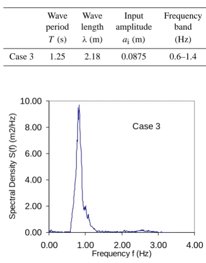
In this work, we adopt the wave tank geometry and set up conditions used in the experimental model described by Ning et al. (2009). An experimental tank was used with the dimensions 69m×3.0mand water depth was set to0.5m. In the study Ning et al. (2009) and Westphalen et al. (2008), four extreme wave cases are investigated with different input amplitudes. Here we reproduce and validate numerically Case 3 only.

In our NWT, the wave characteristics in each case are as shown in Table 1. The length of the numerical tank is the same as the one used by Ning et al. (2009), which is 5 times the characteristic wave length (5λ). In the vertical the tank is set to 1.0 m and the water depth h=0.5 m is the same as in the physical experiments. The width of the tank is taken with a 3 cell layer thickness as 3D, albeit in a narrow numerical tank. In Ning et al. (2009), the parameters used were the focus pointx0=3.27 m and the

focus timet0=10.0 s, respectively. The wave maker signals

for the simulations were calculated using a first and first plus second order formulation and 16 (=N) wave components as recommended by Ning et al. (2009). The corresponding

Table 1. Characteristic waves.

Wave Wave Input Frequency

period length amplitude band T (s) λ(m) ai(m) (Hz)

Case 3 1.25 2.18 0.0875 0.6–1.4

8 Firstly results obtained with the inclusion of first order and first and second order wave

components for comparison with the experimental data of Ning

et al

. (2009) are presented in

Fig. 4, which shows the surface elevation at the focus point. The total number of cells in the

3D domain is 471,900 with a uniform mesh spacing of 0.01667m. The results confirm that

agreement with the experiments up to the time of wave focussing is satisfactory particularly

in the first and second order case, with any discrepancies between experiments and

simulations appearing only after the focal time.

A non-uniform mesh was used for the case with 358×70×3 = 75,180 cells and mesh spacing

in the refined regions of 0.00875m, which gives 10 cells per wave amplitude in the vertical

direction. The results with the inclusion of first order and first and second order simulations

for comparison with the experimental data of Ning

et al

. (2009) are shown in Fig. 5, which

illustrates the surface elevation at the focus point. A comparison of the maximum surface

elevation between simulation and experiments after the focal point (including the focal

point) are shown in Table 2. It can be seen that the first order wave maker signal

underestimates the velocities whilst the results for the first plus second order case provide

reasonable agreement with a fully nonlinear calculation and by implication with the

experimental results. The total CPU time is about 45 hours on one processor of a 600 MHz

NEC vector computer.

Wave

period

T

(s)

Wave length

λ

(m)

Input

amplitude

a

_i

(m)

Frequency Band

(Hz)

Case 3

1.25

2.18 0.0875

0.6-1.4

Table 1 Characteristic waves

Case 3

0.00 2.00 4.00 6.00 8.00 10.00

0.00 1.00 2.00 3.00 4.00

Frequency f (Hz)

S

p

ec

tr

al D

ens

it

y

S

(f

) (

m

2

/H

z

)

Case 3

0.4 0.45 0.5 0.55 0.6

0.00 2.00 4.00 6.00 8.00 10.00 12.00 time (s)

S

u

rf

ac

e el

ev

at

ion

(m

)

First-order Second-order First+Second-order

Fig.1

Input wave spectrum with frequency

Fig.2 Surface elevation at input position

Fig. 1. Input wave spectrum with frequency.

wave spectrum can also be obtained as shown in Fig. 1 by a Fast Fourier Transform.

Firstly results obtained with the inclusion of first order and first and second order wave

components for comparison with the experimental data of Ning

et al

. (2009) are presented in

Fig. 4, which shows the surface elevation at the focus point. The total number of cells in the

3D domain is 471,900 with a uniform mesh spacing of 0.01667m. The results confirm that

agreement with the experiments up to the time of wave focussing is satisfactory particularly

in the first and second order case, with any discrepancies between experiments and

simulations appearing only after the focal time.

A non-uniform mesh was used for the case with 358×70×3 = 75,180 cells and mesh spacing

in the refined regions of 0.00875m, which gives 10 cells per wave amplitude in the vertical

direction. The results with the inclusion of first order and first and second order simulations

for comparison with the experimental data of Ning

et al

. (2009) are shown in Fig. 5, which

illustrates the surface elevation at the focus point. A comparison of the maximum surface

elevation between simulation and experiments after the focal point (including the focal

point) are shown in Table 2. It can be seen that the first order wave maker signal

underestimates the velocities whilst the results for the first plus second order case provide

reasonable agreement with a fully nonlinear calculation and by implication with the

experimental results. The total CPU time is about 45 hours on one processor of a 600 MHz

NEC vector computer.

Wave

period

T

(s)

Wave length

λ

(m)

Input

amplitude

a

_i

(m)

Frequency Band

(Hz)

Case 3

1.25

2.18 0.0875

0.6-1.4

Table 1 Characteristic waves

Case 3

0.00 2.00 4.00 6.00 8.00 10.00

0.00 1.00 2.00 3.00 4.00

Frequency f (Hz)

S

p

ec

tr

al D

ens

it

y

S

(f

) (

m

2

/H

z

)

Case 3

0.4 0.45 0.5 0.55 0.6

0.00 2.00 4.00 6.00 8.00 10.00 12.00

time (s)

S

u

rf

ac

e el

ev

at

ion

(m

)

First-order Second-order First+Second-order

Fig.1

Input wave spectrum with frequency

Fig. 2. Surface elevation at input position.

Fig.2 Surface elevation at input position

At the inflow boundary at the left-side of the tank, the corresponding surface elevations are shown as Fig. 2 and velocities are shown in Fig. 3, where the velocity specification is applied in the water component only and the velocity of the air at the inlet boundary is set to zero. The top boundary and right far boundary are specified with non-reflecting boundary conditions allowing air to leave or enter the domain. The remaining boundaries are set as rigid walls.

(6)

524 Z. Z. Hu et al.: Numerical simulation of floating bodies

Table 2. Maximum surface elevation at wave gauges.

x= 3.27 m x= 3.55 m x= 3.75 m x= 3.95 m

Phys. Exp. by Ning et al. (2009) 0.5967

STAR CCM (1st + 2nd order) by Westphalen et al. (2008) 0.5923 0.5968 0.6007 0.6024

Present result (1st + 2nd order) 0.5931 0.5971 0.6013 0.6026

9

Case 3

-0.60 -0.40 -0.20 0.00 0.20 0.40 0.60 0.80

0.00 2.00 4.00 6.00 8.00 10.00 12.00

time (s)

S

u

rf

ace u

&

w

v

e

lo

c

it

y

(m

/s

)

First-order_u-velocity First+Second-order_u-velocity First-order_v-velocity First+Second-order_v_velocity

Fig.3The horizontal and vertical velocity at input position (x = 0.0m)

Fig.4Comparison of wave elevations at focal point of x=3.27 m

Case 3

0.42 0.46 0.50 0.54 0.58 0.62

6.00 7.00 8.00 9.00 10.00 11.00 12.00 13.00

time (s)

S

u

rf

ac

e e

lev

a

ti

on

(m

)

Physical exp. Result (1st order) Result (1st+2nd order)

x=3.27 m x=3.55 m x=3.75 m x=3.95 m Phys. Exp. By

Ning et. al. (2009)

0.5967

STAR CCM (1st+2nd order) by Westphalen et. al.

(2008)

0.5923 0.5968 0.6007 0.6024

Fig. 3. The horizontal and vertical velocity at input position

(x= 0.0 m).

9

Case 3

-0.60 -0.40 -0.20 0.00 0.20 0.40 0.60 0.80

0.00 2.00 4.00 6.00 8.00 10.00 12.00 time (s)

S

u

rf

ace u

&

w

v

e

lo

c

it

y

(m

/s

)

Case 3

0.42 0.46 0.50 0.54 0.58 0.62

6.00 7.00 8.00 9.00 10.00 11.00 12.00 13.00

time (s)

S

u

rf

ac

e e

lev

a

ti

on

(m

)

Ning et. al. (2009)

0.5967

(2008)

0.5923 0.5968 0.6007 0.6024

Fig. 4. Comparison of wave elevations at focal point ofx= 3.27 m.

Firstly, results obtained with the inclusion of first order and first and second order wave components for comparison with the experimental data of Ning et al. (2009) are presented in Fig. 4, which shows the surface elevation at the focus point. The total number of cells in the 3-D domain is 471 900 with a uniform mesh spacing of 0.01667 m. The results confirm that agreement with the experiments up to the time of wave focussing is satisfactory particularly in the first and second order case, with any discrepancies between experiments and simulations appearing only after the focal time.

A non-uniform mesh was used for the case with 358× 70×3=75180 cells and mesh spacing in the refined regions of 0.00875 m, which gives 10 cells per wave amplitude in the vertical direction. The results with the inclusion of first order and first and second order simulations for comparison with the experimental data of Ning et al. (2009) are shown in Fig. 5, which illustrates the surface elevation at the focus

9

Case 3

-0.60 -0.40 -0.20 0.00 0.20 0.40 0.60 0.80

0.00 2.00 4.00 6.00 8.00 10.00 12.00

time (s)

S

u

rf

ace u

&

w

v

e

lo

c

it

y

(m

/s

)

Case 3

0.42 0.46 0.50 0.54 0.58 0.62

6.00 7.00 8.00 9.00 10.00 11.00 12.00 13.00

time (s)

S

u

rf

ac

e e

lev

a

ti

on

(m

)

Ning et. al. (2009)

0.5967

(2008)

0.5923 0.5968 0.6007 0.6024

Fig. 5. Comparison of wave elevations at focal point ofx= 3.27 m.

point. A comparison of the maximum surface elevation between simulation and experiments after the focal point (including the focal point) are shown in Table 2. It can be seen that the first order wave maker signal underestimates the velocities whilst the results for the first plus second order case provide reasonable agreement with a fully nonlinear calculation and by implication with the experimental results. The total CPU time is about 45 h on one processor of a 600 MHz NEC vector computer.

6.2 A fixed horizontal cylinder in regular waves

The case next considered is the interaction between regular waves and a half submerged horizontal cylinder in a tank. The purpose of the test case is to provide validation of the wave forces acting on the cylinder compared with the theory based on Morison’s equation and experimental results (see Dixon et al., 1979; Easson et al., 1985). To correspond with the physical experiments, first-order regular waves are generated in a tank to interact with the cylinder. The inflow boundary velocity componentsu,wand the surface elevation ηare

u= gAkcosh(k (z+h))cos(kx−ωt ) ωcosh(kh)

v= gAksinh(k (z+h))sin(kx−ωt ) ωcosh(kh)

η=Acos(kx−ωt )

with the velocity specification applied in the water compo-nent only and the velocity of the air at the inlet boundary set to zero. The top boundary and right far boundary are

(7)

Z. Z. Hu et al.: Numerical simulation of floating bodies 525

10 Present result

(1

st

+2

nd

order)

0.5931 0.5971 0.6013

0.6026

Table 2 Maximum surface elevation at wave gauges

6.2. A fixed horizontal cylinder in regular waves

The case next considered is the interaction between regular waves and a half submerged

horizontal cylinder in a tank. The purpose of the test case is to provide validation of the

wave forces acting on the cylinder compared with the theory based on Morison’s equation

and experimental results (see Dixon

et al

. (1979) and Easson

et al

. (1985)). To correspond

with the physical experiments first-order regular waves are generated in a tank to interact

with the cylinder. The inflow boundary velocity components

u

,

w

and the surface elevation

η

are

)

cosh(

)

cos(

))

(

cosh(

kh

t

kx

h

z

k

gAk

u

ω

−

+

=

)

cosh(

)

sin(

))

(

sinh(

kh

t

kx

h

z

k

gAk

v

ω

−

+

=

η

=

A

cos(

kx

−

ω

t

)

with the velocity specification applied in the water component only and the velocity of the

air at the inlet boundary set to zero.

The top boundary and right far boundary are specified

using non-reflecting boundary conditions allowing air to leave or enter the domain. The

remaining boundaries are set as rigid walls.

The NWT geometry used had outer dimensions 12 m

×

1.5 m

×

0.21 m and the water depth

used was

h

=

1 .

0 m

. The position of the cylinder was set about one wave period (wave length

of

3 .

90 m

) from the wave maker (see Figs.6 &7). A non-uniform mesh was used for the case

with 475×69×14 = 458,850 cells and mesh spacing in the refined regions = 0.015m as

shown in Fig.8. The set up parameters are: cylinder diameter,

D

=

0 .

25 m

, length of cylinder

m

l

=

0 .

12 ,

wave amplitude

A

=

0 .

125 m

, wave frequency

ω

=

3 .

817 and

k

=

1 .

61 . Fig.9

shows time histories of the relative vertical force over one period, which relative force

defines to

F

'

=

F

_z

/[

g

ρ

(

π

D

2

l

/

4 )]

and

F

_z

is a force on the cylinder resulting from the

pressure acting on the surface calculated in the vertical direction. It can be seen that good

agreement is achieved with the experimental data and theoretical forces providing

satisfactory evidence of the accuracy of the present model.

Fig.6 A horizontal cylinder Fig.7 A horizontal cylinder in the NWT

Fig. 6. A horizontal cylinder.

10 Present result

(1

st

+2

nd

order)

0.5931 0.5971 0.6013

0.6026

Table 2 Maximum surface elevation at wave gauges

6.2. A fixed horizontal cylinder in regular waves

The case next considered is the interaction between regular waves and a half submerged

horizontal cylinder in a tank. The purpose of the test case is to provide validation of the

wave forces acting on the cylinder compared with the theory based on Morison’s equation

and experimental results (see Dixon

et al

. (1979) and Easson

et al

. (1985)). To correspond

with the physical experiments first-order regular waves are generated in a tank to interact

with the cylinder. The inflow boundary velocity components

u

,

w

and the surface elevation

η

are

)

cosh(

)

cos(

))

(

cosh(

kh

t

kx

h

z

k

gAk

u

ω

−

+

=

)

cosh(

)

sin(

))

(

sinh(

kh

t

kx

h

z

k

gAk

v

ω

−

+

=

η

=

A

cos(

kx

−

ω

t

)

with the velocity specification applied in the water component only and the velocity of the

air at the inlet boundary set to zero.

The top boundary and right far boundary are specified

using non-reflecting boundary conditions allowing air to leave or enter the domain. The

remaining boundaries are set as rigid walls.

The NWT geometry used had outer dimensions 12 m ×1.5 m ×

0.21 m and the water depth

used was

h=1.0m

. The position of the cylinder was set about one wave period (wave length

of

3.90m

) from the wave maker (see Figs.6 &7). A non-uniform mesh was used for the case

with 475×69×14 = 458,850 cells and mesh spacing in the refined regions = 0.015m as

shown in Fig.8. The set up parameters are: cylinder diameter,

D=0.25m

, length of cylinder

m

l =0.12

,

wave amplitude

A=0.125m

, wave frequency

ω

=3.817

and

k=1.61

. Fig.9

shows time histories of the relative vertical force over one period, which relative force

defines to

F

'

=

F

z

/[

g

ρ

(

π

D

2

l

/

4 )]

and

Fz

is a force on the cylinder resulting from the

pressure acting on the surface calculated in the vertical direction. It can be seen that good

agreement is achieved with the experimental data and theoretical forces providing

satisfactory evidence of the accuracy of the present model.

Fig.6 A horizontal cylinder Fig.7 A horizontal cylinder in the NWT

Fig. 7. A horizontal cylinder in the NWT.

specified using non-reflecting boundary conditions allowing air to leave or enter the domain. The remaining boundaries are set as rigid walls.

The NWT geometry used had outer dimensions 12 m×1.5 m×0.21 m and the water depth used was h=1.0 m. The position of the cylinder was set about one wave period (wave length of 3.90 m) from the wave maker (see Figs. 6 and 7). A non-uniform mesh was used for the case with 475×69×14=458850 cells and mesh spacing in the refined regions = 0.015 m as shown in Fig. 8. The set up parameters are: cylinder diameter, D=0.25 m, length of cylinderl=0.12 m, wave amplitudeA=0.125 m, wave frequency ω=3.817 and k=1.61. Figure 9 shows time histories of the relative vertical force over one period, which relative force defines toF0=Fz/gρ π D2l/4andFzis a force on the cylinder resulting from the pressure acting on the surface calculated in the vertical direction. It can be seen that good agreement is achieved with the experimental data and theoretical forces providing satisfactory evidence of the accuracy of the present model.

6.3 Wave interaction with the floating Bobber in the tank

The NWT domain for this extreme waves case is 13 m×1.0 m×0.48 m with a water depth for the tests of h=0.5 m. The geometry of the Bobber is as follows: the diameter of the hemispherical base is 0.3 m, the vertical sides extend to a flat top 0.15 m above the curved section. The initial position of the apex of the Bobber geometry in the tank is at the wave focus point 3.0 m×0.24 m×0.35 m and a non-uniform mesh is used with 425×40×22=374000 cells and refined regions with local mesh spacing of 0.02 m around the

11 Fig.8

Cartesian cut cell mesh around Fig.9

Relative vertical forces on horizontal

horizontal cylinder cylinder

6.3 Wave Interaction with the floating Bobber in the tank

The NWT domain for this extreme waves case is

13 m

×

1 .

0 m

×

0 .

48 m

with a water depth for

the tests of

h

=

0 .

5 m

. The geometry of the Bobber is as follows: the diameter of the

hemispherical base is 0.3m, the vertical sides extend to a flat top 0.15m above the curved

section. The initial position of the apex of the Bobber geometry in the tank is at the wave

focus point 3.0m×0.24m×0.35m and a non-uniform mesh is used with 425×40×22 = 374,000

cells and refined regions with local mesh spacing of 0.02m around the geometry (see Figs.

10 & 11). The focus time, focus point and the input wave amplitude are set up in the same

manner as before in the empty tank. Reflection boundary conditions are used on the Bobber

boundary and the other boundaries are specified in the same manner as in the case of the

empty NWT.

The mass of the Bobber geometry is taken as the volume of the hemispherical base. The

Bobber geometry is allowed to articulate in heave motion only, responding to the wave

excitation, while all other modes are restrained. As expected, the response is in terms of the

vertical velocity, displacement and heave displacement of the Bobber geometry. The

corresponding results for the free surface elevation on the front side of the Bobber geometry

is shown in Fig. 12; the heave force on the Bobber geometry is shown in Fig. 13; the vertical

velocity in Fig. 14, and the heave displacement of the Bobber geometry is shown in Fig. 15.

Fig. 16 illustrates the wave profile around the Bobber geometry. These results include the

incoming wave, diffracted wave, radiated wave and the wave created by the heave motion of

the body.

Fig. 10 The Bobber geometry Fig. 11 The Bobber in the NWT

-0.60 -0.40 -0.20 0.00 0.20 0.40

0.00 0.50 1.00

t/T

R

e

la

ti

ve

rt

ic

a

l

fo

rc

e

Theoretical force

Experimental force

Present result

Fig. 8. Cartesian cut cell mesh around horizontal cylinder.

Fig.8

Cartesian cut cell mesh around Fig.9

Relative vertical forces on horizontal

horizontal cylinder cylinder

6.3 Wave Interaction with the floating Bobber in the tank

The NWT domain for this extreme waves case is

13 m

×

1 .

0 m

×

0 .

48 m

with a water depth for

the tests of

h

=

0 .

5 m

. The geometry of the Bobber is as follows: the diameter of the

hemispherical base is 0.3m, the vertical sides extend to a flat top 0.15m above the curved

section. The initial position of the apex of the Bobber geometry in the tank is at the wave

focus point 3.0m×0.24m×0.35m and a non-uniform mesh is used with 425×40×22 = 374,000

cells and refined regions with local mesh spacing of 0.02m around the geometry (see Figs.

10 & 11). The focus time, focus point and the input wave amplitude are set up in the same

manner as before in the empty tank. Reflection boundary conditions are used on the Bobber

boundary and the other boundaries are specified in the same manner as in the case of the

empty NWT.

The mass of the Bobber geometry is taken as the volume of the hemispherical base. The

Bobber geometry is allowed to articulate in heave motion only, responding to the wave

excitation, while all other modes are restrained. As expected, the response is in terms of the

vertical velocity, displacement and heave displacement of the Bobber geometry. The

corresponding results for the free surface elevation on the front side of the Bobber geometry

is shown in Fig. 12; the heave force on the Bobber geometry is shown in Fig. 13; the vertical

velocity in Fig. 14, and the heave displacement of the Bobber geometry is shown in Fig. 15.

Fig. 16 illustrates the wave profile around the Bobber geometry. These results include the

incoming wave, diffracted wave, radiated wave and the wave created by the heave motion of

the body.

Fig. 10 The Bobber geometry Fig. 11 The Bobber in the NWT

-0.60 -0.40 -0.20 0.00 0.20 0.40

0.00 0.50 1.00

t/T

R

e

la

ti

ve

rt

ic

a

l

fo

rc

e

Theoretical force

Experimental force

Present result

Fig. 9. Relative vertical forces on horizontal cylinder.

11 Fig.8

Cartesian cut cell mesh around Fig.9

Relative vertical forces on horizontal

horizontal cylinder cylinder

6.3 Wave Interaction with the floating Bobber in the tank

The NWT domain for this extreme waves case is

13 m

×

1 .

0 m

×

0 .

48 m

with a water depth for

the tests of

h

=

0 .

5 m

. The geometry of the Bobber is as follows: the diameter of the

hemispherical base is 0.3m, the vertical sides extend to a flat top 0.15m above the curved

section. The initial position of the apex of the Bobber geometry in the tank is at the wave

focus point 3.0m×0.24m×0.35m and a non-uniform mesh is used with 425×40×22 = 374,000

cells and refined regions with local mesh spacing of 0.02m around the geometry (see Figs.

10 & 11). The focus time, focus point and the input wave amplitude are set up in the same

manner as before in the empty tank. Reflection boundary conditions are used on the Bobber

boundary and the other boundaries are specified in the same manner as in the case of the

empty NWT.

The mass of the Bobber geometry is taken as the volume of the hemispherical base. The

Bobber geometry is allowed to articulate in heave motion only, responding to the wave

excitation, while all other modes are restrained. As expected, the response is in terms of the

vertical velocity, displacement and heave displacement of the Bobber geometry. The

corresponding results for the free surface elevation on the front side of the Bobber geometry

is shown in Fig. 12; the heave force on the Bobber geometry is shown in Fig. 13; the vertical

velocity in Fig. 14, and the heave displacement of the Bobber geometry is shown in Fig. 15.

Fig. 16 illustrates the wave profile around the Bobber geometry. These results include the

incoming wave, diffracted wave, radiated wave and the wave created by the heave motion of

the body.

Fig. 10 The Bobber geometry Fig. 11 The Bobber in the NWT

-0.60 -0.40 -0.20 0.00 0.20 0.40

0.00 0.50 1.00

t/T

R

e

la

ti

ve

rt

ic

a

l

fo

rc

e

Theoretical force

Experimental force

Present result

Fig. 10. The Bobber geometry.

geometry (see Figs. 10 and 11). The focus time, focus point and the input wave amplitude are set up in the same manner as before in the empty tank. Reflection boundary conditions are used on the Bobber boundary and the other boundaries are specified in the same manner as in the case of the empty NWT.

The mass of the Bobber geometry is taken as the volume of the hemispherical base. The Bobber geometry is allowed to articulate in heave motion only, responding to the wave excitation, while all other modes are restrained. As expected, the response is in terms of the vertical velocity, displacement and heave displacement of the Bobber geometry. The corresponding results for the free surface elevation on the front side of the Bobber geometry is shown in Fig. 12; the

(8)

526 Z. Z. Hu et al.: Numerical simulation of floating bodies

11 Fig.8

Cartesian cut cell mesh around Fig.9

Relative vertical forces on horizontal

horizontal cylinder cylinder

6.3 Wave Interaction with the floating Bobber in the tank

The NWT domain for this extreme waves case is

13 m

×

1 .

0 m

×

0 .

48 m

with a water depth for

the tests of

h

=

0 .

5 m

. The geometry of the Bobber is as follows: the diameter of the

hemispherical base is 0.3m, the vertical sides extend to a flat top 0.15m above the curved

section. The initial position of the apex of the Bobber geometry in the tank is at the wave

focus point 3.0m×0.24m×0.35m and a non-uniform mesh is used with 425×40×22 = 374,000

cells and refined regions with local mesh spacing of 0.02m around the geometry (see Figs.

10 & 11). The focus time, focus point and the input wave amplitude are set up in the same

manner as before in the empty tank. Reflection boundary conditions are used on the Bobber

boundary and the other boundaries are specified in the same manner as in the case of the

empty NWT.

The mass of the Bobber geometry is taken as the volume of the hemispherical base. The

Bobber geometry is allowed to articulate in heave motion only, responding to the wave

excitation, while all other modes are restrained. As expected, the response is in terms of the

vertical velocity, displacement and heave displacement of the Bobber geometry. The

corresponding results for the free surface elevation on the front side of the Bobber geometry

is shown in Fig. 12; the heave force on the Bobber geometry is shown in Fig. 13; the vertical

velocity in Fig. 14, and the heave displacement of the Bobber geometry is shown in Fig. 15.

Fig. 16 illustrates the wave profile around the Bobber geometry. These results include the

incoming wave, diffracted wave, radiated wave and the wave created by the heave motion of

the body.

Fig. 10 The Bobber geometry Fig. 11 The Bobber in the NWT

-0.60 -0.40 -0.20 0.00 0.20 0.40

0.00 0.50 1.00

t/T R e la ti ve ve rt ic a l fo rc e Theoretical force Experimental force Present result

Fig. 11. The Bobber in the NWT.

12 Case 3

40 45 50 55 0.60 0.65

0.00 4.00 8.00 12.00 time (s) l v ti n m ) e ( c a 0. f o r

Su a0._e e0. 0.

Case 3

-30.00 -20.00 -10.00 0.00 10.00 20.00 30.00

0.00 4.00 _{time (s)} 8.00 12.00

He a v e fo rc e (N)

Fig.12 Time history of wave run-up on the Fig.13 Time history of the heave force

front side of the Bobber geometry on the Bobber geometry

Case 3

-0.60 -0.30 0.00 0.30 0.60

0.00 4.00 8.00 12.00 time (s) V e rt ic a l v e lo c it y (m /s )

Case 3

-0.10 -0.05 0.00 0.05 0.10

0.00

4.00

8.00

12.00

time (s) Ve rt ic a l d isp la ce m e n t (m )

Fig.14 Time history of the vertical velocity Fig.15 Time history of the displacement

of the Bobber geometry of the Bobber geometry

Fig.16 Wave profile around the Bobber

7. Conclusions

A numerical tank with free surface capturing and Cartesian cut cell method has being

modified and developed for the simulation of wave energy devices under modelled extreme

wave conditions. The results show the emerging promise of the NWT for the simulation of

nonlinear wave interactions with fixed and floating bodies. Future work will include

extensions to other wave energy converter devices admitting a full complement of degrees

of freedom as opposed to heave alone as considered here, and to wave interactions with

other floating bodies and fixed structures including aeration of the water component under

violent wave impact situations.

8. Acknowledgements

This work was supported by the UK Engineering and Physical Sciences Research Council

(EPSRC) (ref. EP/D077621) for which the authors are most grateful.

References

Fig. 12. Time history of wave run-up on the front side of the Bobber

geometry.

12 Case 3

0.40

0.45

0.50

0.55

0.60

0.65

0.00

4.00

8.00

12.00 time (s)

Su

rf

a

c

e

le

v

a

ti

o

n

(m

)

Case 3

-30.00 -20.00 -10.00 0.00 10.00 20.00 30.00

0.00 4.00 _{time (s)} 8.00 12.00

He a v e fo rc e (N )

Fig.12 Time history of wave run-up on the Fig.13 Time history of the heave force

front side of the Bobber geometry on the Bobber geometry

Case 3

-0.60

-0.30

0.00

0.30

0.60

0.00

4.00

8.00

12.00 time (s)

V

e

rt

ic

a

l v

e

lo

c

it

y

(m

/s

)

Case 3

-0.10

-0.05

0.00

0.05

0.10

0.00

4.00

8.00

12.00 time (s)

Ve

rt

ic

a

l

d

isp

la

ce

m

e

n

t

(m

)

Fig.14 Time history of the vertical velocity Fig.15 Time history of the displacement

of the Bobber geometry of the Bobber geometry

Fig.16 Wave profile around the Bobber

7. Conclusions

A numerical tank with free surface capturing and Cartesian cut cell method has being

modified and developed for the simulation of wave energy devices under modelled extreme

wave conditions. The results show the emerging promise of the NWT for the simulation of

nonlinear wave interactions with fixed and floating bodies. Future work will include

extensions to other wave energy converter devices admitting a full complement of degrees

of freedom as opposed to heave alone as considered here, and to wave interactions with

other floating bodies and fixed structures including aeration of the water component under

violent wave impact situations.

8. Acknowledgements

This work was supported by the UK Engineering and Physical Sciences Research Council

(EPSRC) (ref. EP/D077621) for which the authors are most grateful.

References

Fig. 13. Time history of the heave force on the Bobber geometry.

12 Case 3

0.40

0.45

0.50

0.55

0.60

0.65

0.00

4.00

8.00

12.00 time (s)

Su

rf

a

c

e

le

v

a

ti

o

n

(m

)

Case 3

-30.00

-20.00

-10.00

0.00

10.00

20.00

30.00

0.00

4.00 _{time (s)}

8.00

12.00 He

a

v

e

fo

rc

e

(N

)

Fig.12 Time history of wave run-up on the Fig.13 Time history of the heave force

front side of the Bobber geometry on the Bobber geometry

Case 3

-0.60

-0.30

0.00

0.30

0.60

0.00

4.00

8.00

12.00 time (s)

V

e

rt

ic

a

l v

e

lo

c

it

y

(m

/s

)

Case 3

-0.10

-0.05

0.00

0.05

0.10

0.00

4.00

8.00

12.00 time (s)

Ve

rt

ic

a

l

d

isp

la

ce

m

e

n

t

(m

)

Fig.14 Time history of the vertical velocity Fig.15 Time history of the displacement

of the Bobber geometry of the Bobber geometry

Fig.16 Wave profile around the Bobber

7. Conclusions

A numerical tank with free surface capturing and Cartesian cut cell method has being

modified and developed for the simulation of wave energy devices under modelled extreme

wave conditions. The results show the emerging promise of the NWT for the simulation of

nonlinear wave interactions with fixed and floating bodies. Future work will include

extensions to other wave energy converter devices admitting a full complement of degrees

of freedom as opposed to heave alone as considered here, and to wave interactions with

other floating bodies and fixed structures including aeration of the water component under

violent wave impact situations.

8. Acknowledgements

This work was supported by the UK Engineering and Physical Sciences Research Council

(EPSRC) (ref. EP/D077621) for which the authors are most grateful.

References

Fig. 14. Time history of the vertical velocity of the Bobber

geometry.

12 Case 3

0.40

0.45

0.50

0.55

0.60

0.65

0.00

4.00

8.00

12.00 time (s)

Su

rf

a

c

e

le

v

a

ti

o

n

(m

)

Case 3

-30.00 -20.00 -10.00 0.00 10.00 20.00 30.00

0.00 4.00 _{time (s)} 8.00 12.00

Fig.12 Time history of wave run-up on the Fig.13 Time history of the heave force

front side of the Bobber geometry on the Bobber geometry

Case 3

-0.60 -0.30 0.00 0.30 0.60

0.00 4.00 8.00 12.00 time (s) V e rt ic a l v e lo c it y (m /s )

Case 3

-0.10

-0.05

0.00

0.05

0.10

0.00

4.00 _{time (s)}

8.00

12.00 Ve

rt

ic

a

l

d

isp

la

ce

m

e

n

t

(m

)

Fig.14 Time history of the vertical velocity Fig.15 Time history of the displacement

of the Bobber geometry of the Bobber geometry

Fig.16 Wave profile around the Bobber

7. Conclusions

A numerical tank with free surface capturing and Cartesian cut cell method has being

modified and developed for the simulation of wave energy devices under modelled extreme

wave conditions. The results show the emerging promise of the NWT for the simulation of

nonlinear wave interactions with fixed and floating bodies. Future work will include

extensions to other wave energy converter devices admitting a full complement of degrees

of freedom as opposed to heave alone as considered here, and to wave interactions with

other floating bodies and fixed structures including aeration of the water component under

violent wave impact situations.

8. Acknowledgements

This work was supported by the UK Engineering and Physical Sciences Research Council

(EPSRC) (ref. EP/D077621) for which the authors are most grateful.

References

Fig. 15. Time history of the displacement of the Bobber geometry.

12

Case 3 0.40 0.45 0.50 0.55 0.60 0.65

0.00 4.00 8.00 12.00

time (s) Su rf a c e e le v a ti o n (m ) Case 3 -30.00 -20.00 -10.00 0.00 10.00 20.00 30.00

0.00 4.00 _{time (s)} 8.00 12.00

Fig.12 Time history of wave run-up on the Fig.13 Time history of the heave force

front side of the Bobber geometry on the Bobber geometry

Case 3 -0.60 -0.30 0.00 0.30 0.60

0.00 4.00 8.00 12.00

time (s) V e rt ic a l v e lo c it y (m /s ) Case 3 -0.10 -0.05 0.00 0.05 0.10

0.00 4.00 _{time (s)} 8.00 12.00

Ve rt ic a l d isp la ce m e n t (m )

Fig.14 Time history of the vertical velocity Fig.15 Time history of the displacement

of the Bobber geometry of the Bobber geometry

Fig.16 Wave profile around the Bobber

7. Conclusions

A numerical tank with free surface capturing and Cartesian cut cell method has being

modified and developed for the simulation of wave energy devices under modelled extreme

wave conditions. The results show the emerging promise of the NWT for the simulation of

nonlinear wave interactions with fixed and floating bodies. Future work will include

extensions to other wave energy converter devices admitting a full complement of degrees

of freedom as opposed to heave alone as considered here, and to wave interactions with

other floating bodies and fixed structures including aeration of the water component under

violent wave impact situations.

8. Acknowledgements

This work was supported by the UK Engineering and Physical Sciences Research Council

(EPSRC) (ref. EP/D077621) for which the authors are most grateful.

References

Fig. 16. Wave profile around the Bobber.

heave force on the Bobber geometry is shown in Fig. 13; the vertical velocity in Fig. 14, and the heave displacement of the Bobber geometry is shown in Fig. 15. Figure 16 illustrates the wave profile around the Bobber geometry. These results include the incoming wave, diffracted wave, radiated wave and the wave created by the heave motion of the body.

7 Conclusions

A numerical tank with free surface capturing and Cartesian cut cell method has been modified and developed for the simulation of wave energy devices under modelled extreme wave conditions. The results show the emerging promise of the NWT for the simulation of nonlinear wave interactions with fixed and floating bodies. Future work will include extensions to other wave energy converter devices admitting a full complement of degrees of freedom as opposed to heaving alone as considered here, and to wave interactions with other floating bodies and fixed structures including aeration of the water component under violent wave impact situations.

Acknowledgements. This work was supported by the UK Engineering and Physical Sciences Research Council (EPSRC) (ref. EP/D077621) for which the authors are most grateful.

Edited by: E. Pelinovsky

Reviewed by: two anonymous referees

(9)

References

Causon, D. M., Ingram, D. M., Mingham, C. G., Yang, G., and Pearson, R. V.: Calculation of shallow water flows using a Cartesian cut cell approach, Adv. Water Resour., 23, 545–562, 2000.

Causon, D. M., Ingram, D. M., and Mingham, C. G.: A Cartesian cut cell method for shallow water flows with moving boundaries, Adv. Water Resour., 24, 899–911, 2001.

Dalzell, J. F.: A note on finite depth second-order wave-wave interactions, Appl. Ocean Res., 21, 105–111, 1999.

Dixon, A. G., Greated, A., and Salter, S. H.: Wave forces on partially submerged cylinders, J. Waterw. Port. C.-ASCE, 105(4), 421–438, 1979.

Easson, W. J., Greated, C. A., and Duranni, T. S.: Force spectra from partially submerged circular cylinders in random seas, J. Waterw. Port. C.-ASCE, 111(5), 856–879, 1985.

Hu, Z. Z., Causon, D. M., Mingham, C. M., and Qian, L.: Numerical wave tank study of a wave energy converter in heave, Proceedings 19th ISOPE conference, Osaka, Japan, 383–388, 2009.

Ning, D. Z., Zang, J., Liu, S. X., Taylor, R. E., Teng, B., and Taylor, P. H.: Free surface and wave kinematics for nonlinear focused wave groups, Ocean Eng., 36(15–16), 1226–1243, 2009. Qian, L., Causon, D. M., Ingram, D. M., and Mingham, C. G.:

Cartesian cut cell two fluid solver for hydraulic flow problems, J. Hydraul. Eng.-ASCE, 129(9), 688–696, 2003.

Qian, L., Causon, D. M. Mingham, C. G., and Ingram, D. M.: A Free-Surface Capturing Method for Two Fluid Flows with Moving Bodies, P. Roy. Soc. A-Math. Phy., 462(2065), 21–42, 2006.

Yang, G., Causon, D. M., Ingram, D. M., Saunders, R., and Batten, P.: A Cartesian cut cell method for compressible flows – Part A: static body problems, Aeronaut. J., 101(1002), 47–56, 1997. Yang, G., Causon, D. M., and Ingram, D. M.: A Calculation of

compressible flows about complex moving geometries using a 3D Cartesian cut cell method, Int. J. Numer. Meth. F., 33, 1121– 1151, 2000.