OPTIMAL SIZING OF DG UNITS
USING EXACT LOSS FORMULA AT
OPTIMAL POWER FACTOR
P.Sobha Rani*
Electrical and Electronics Engineering department N.B.K.R.Institute of Science&Technology
Vidyanagar, Andhra Pradesh E mail id:[email protected]
Dr.A.Lakshmi Devi*
Elecrical Engineering department s.v.u.college of engineering, Tirupati.
E mail id:[email protected]
ABSTRACT
Distributed generators are beneficial in reducing the losses effectively compared to other methods of loss reduction. The challenge of identifying the optimal locations and sizes of DG has generated research interests all over the world and many efforts have been made in this direction. Studies have indicated that inappropriate locations and sizes of DG may lead to higher system losses than the ones in the existing network. In this paper IEEE 33-bus system is selected for locating and sizing of optimal distributed generation source. The DG unit size is calculated using exact loss formula. With the optimal size of DG unit at a suitable location and at optimal power factor, it resulted in reduction in power losses and improvement in voltage profile.
Key words: distributed generation, load-flow, power factor
1. INTRODUCTION
Distribution system provides a final link between the high voltage transmission and consumers. A radial distribution system has main feeders and lateral distributors. The main feeder originates from substation and passes through different consumer loads. Laterals are connected to individual loads. Generally radial distribution systems are used because of their simplicity. Power loss in a distribution system is high because of low voltage and hence high current. The overall efficiency can be improved using DG units. DG is increasingly drawing great attention and development of DGs will bring new chances to traditional distribution systems. However, installation of DG in non-optimal places can result in increasing system losses, voltage problems etc. The beneficial effects of DG mainly depend on its location and size. Selection of optimal location and size of DG is a necessary process to maintain the reliability and stability of existing system effectively before it is connected to power grid.
This paper presents a load flow based method to determine the optimal location to place a DG unit in radial systems to improve the voltage profile of the entire system. The exact location and size of DG is calculated by using exact loss formula. Using exact loss formula sensitivity factors are calculated and bus with highest sensitivity factor is selected as bus with highest power loss. The algorithm is tested on an IEEE 33-bus distribution system.
2. Load flow study
The Power flow problem is a set of simultaneous non linear algebraic equations. Hence numericaltechniques are required to solve this set of equations. The acceptable load flow analysis method should have high speed, low storage requirements, reliable and have acceptable versatility and simplicity The proposed approach utilizes forward and backward sweep algorithm based on KCL and KVL for evaluating the node voltages iteratively. In this approach, computation of branch current depends only on the current injected at the
neighboring node and the current in the adjacent branch. This approach starts from the end nodes of sub lateral line, lateral line and main line and moves towards the root node during branch current computation. The node voltage evaluation begins from the root node and moves towards the nodes located at the far end of the main, lateral and sub lateral lines
.
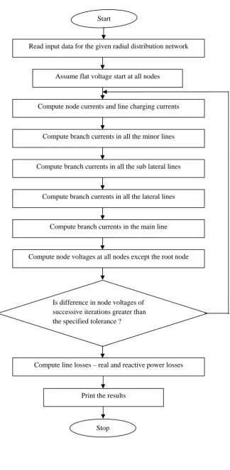
The flow chart shown in Fig.1 depicts the step-by-step procedure of the proposedRead input data for the given radial distribution network
Assume flat voltage start at all nodes Start
Compute node currents and line charging currents
Compute branch currents in all the minor lines
Compute branch currents in all the sub lateral lines
Compute branch currents in all the lateral lines
Compute branch currents in the main line
Compute node voltages at all nodes except the root node
Is difference in node voltages of successive iterations greater than the specified tolerance ?
Compute line losses – real and reactive power losses
Print the results
Stop
3.Methodology
In a large transmission system network with high power losses, it is difficult to select a particular bus from many buses so as to place a DG unit for loss reduction. Power losses are present at every bus and identification of bus with highest power loss is important because losses at that bus includes majority of total sses in the system .The cost of power transmission is reduced by minimizing power losses. This can be partially accomplished by DG unit placement in the network. If DG size exceeds certain value of limit, power loss at that bus becomes negative. This situation must be avoided.
3.1 Identification of optimal DG size
DG can be classified into four major types based on their terminal characteristics in terms of real and reactive power delivering capability as follows:
1. DG capable of injecting P only.
2. DG capable of injecting Q only.
3. DG capable of injecting both P and Q.
4. DG capable of injecting P but consuming Q.
Photovoltaic, micro turbines, fuel cells which are integrated to main grid with the help of converters and inverters are good examples of Type1.Type2 could be synchronous compensators such as gas turbines. DG units that are based on synchronous machines fall in Type3. Type4 is mainly induction generators that are used in wind farms.
The power loss is given by
nj i
j i j i ij j i j i ij
L
P
P
Q
Q
Q
P
P
Q
P
1 , 1
)]
(
)
(
[
(1)where
(
i j)
j i
ij
ij
Cos
V
V
r
(2)and
(
i j)
j i
ij
ij
Sin
V
V
r
(3)Assuming a = (sign) tan (cos-1 (PFDG)), the reactive power output of DG is
QDGi = a PDGi ……… (4)
in which
sign = +1: DG injecting reactive power;
sign = -1: DG consuming reactive power:
PFDG is the Power factor of DG.
The active and reactive power injected at bus i, where the DG located, are given by
Pi = PDGi – PDi ………(5)
Qi = QDGi – QDi = aPDGi – QDi ……….(6)
n j j j ij j j ij GiL
P
aQ
aP
Q
P
P
10
)]
(
)
(
[
*
2
(7)From (1), (5), (6),
0
)
(
)
(
DGi
Di
2 DGi
Di
ii Di
Di
i
i
ii
P
P
a
P
aQ
Q
aP
X
aY
(8)From (8), the optimal size of DG at each bus i for minimizing loss can be written as
ii ii i i Di Di ii Di Di ii DGi
a
aY
X
Q
aP
Q
P
P
2)
(
)
(
(9)In the above expression PDGI gives the optimal capacity of DG unit to be placed in transmission system.
DGI gives the optimal capacity of DG unit to be placed in transmission system.
The power factor of DG depends on operating conditions and type of DG. When the power factor of DG is given, the optimal sizeof DG at each bus i for minimizing losses can be found in the following way.
Type 1 DG: For Type 1 DG, power factor is at unity, i.e., PFDG = 1, a = 0. From (9), the optimal size of DG at
each bus i for minimizing losses can be given by reduced equation
n i j i j ij j ij j i ii ii DiDGi
P
Q
P
Q
P
,
)]
(
[
1
Type 2 DG: Assuming PFDG = 0 and a = ∞, from (9), the optimal size of DG at each bus i for minimizing losses
is given by reduced equation (10)
n i j i j ij j ij j i ii ii DiDGi
Q
P
Q
P
Q
,
)]
(
[
1
(10)3) Type 3 DG: Assuming 0 < PFDG < 1, sign = +l and "a" is a constant, the optimal size of DG at each bus i for
the minimum loss is given by (9) and (6), respectively
4) Type 4 DG: Assuming 0 < PFDG < l, sign = -1 and "a" is a constant, the optimal size of DG at each bus i for
the minimum loss is given by (9) and (5), respectively
3.2 Optimal Location
For optimal location, first the optimal sizes at various locations have been calculated for different types of DG and the losses were calculated with optimal sizes for each case. The case with minimum losses is selected as the optimal location for each type of DG. Based on this method, one can avoid exhaustive computation and save time, especially for large-scale distribution systems as trend of loss with
α and β coefficients from the bases case
3.2.1 .Optimal Power Factor
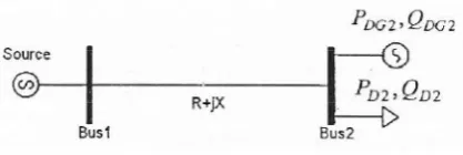
Consider a simple distribution system with two buses, a source, a load and DG connected through a transmission line as shown in Fig.2.
The power factor of the single load (PFD2 ) is given by (11)
2 2 2
2 2 2
D D
D D
Q
P
P
PF
(11)It can be proved that at the minimum loss occur when power factor of DG is equal to the power factor of load as given by (9).
2 2 2
2 2 2
2
DG DG
DG DG
D
Q
P
P
PF
PF
To find the optimal power factor of DG for a radial complex distribution system, fast and repeated methods are proposed. It is interesting to note that in all the three test systems the optimal power factor of DG (Type 3) placed for loss reduction found to be closer to the power factor of combined load of respective system
3.3 Computational Procedure
When power factor of DG is set to be equal to that of combined total loads, computational procedure to find optimal size and location of one of four types of DGs is described in the following.
Step l: Run load flow for the base case.
Step 2: Find the base case loss
Step 3: Calculate power factor of DG using (9).
Step 4: Find the optimal size of DG for each bus using (4) and (10).
Step 5: Place DG with the optin1al size obtained in step 4 at each bus, one at atime. Calculate the approximate loss for each case using (1) with the values α and β of the base case
Step 6: Locate the optimal bus at which the total loss is minimum corresponding with the optimal size at that bus.
Step 7: Run load flow with the optimal size at the optimal, location obtained in step 6. Calculate the exact loss using (1) and the values α and β after DG placement.
It is noted that when the type and power factor of DG is given; the computational procedure to find the optimal size and location of DG is as described earlier apart from step 3. At this step, the power factor of DG is entered rather than using (17). In Exhaustive Load Flow (ELF) method, optimal location and power factor are obtained with a number of load flow solutions.
4. SIMULATION
The proposed method of loss reduction by DG unit placement was tested on a distribution system consisting of 33 buses. Optimal sizes of DG units are calculated at each and every bus. Though the proposed methods can handle four different types of DG units, results of type3 DG units are presented. The optimal power factor is 0.83. Bus8 is selected as optimal location as the losses are minimum compared to all other buses.
Figure1:Optimal DG sizes at all buses for IEEE 33 Bus system
Figure2 shows graphical representation of system total real power loss with optimum DGs at all buses with optimal DGs placed at each bus. The lowest value of loss is around 140kw.DGof size 0.932MVA is placed at bus8.
Figure2:System Total real power loss with optimum DGs at all buses.
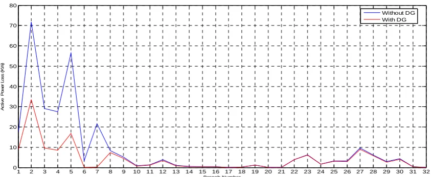
Figure 3. Shows line active power loss with DG at bus 8 and without DG. The losses are reduced and it can be seen as difference between the lines blue and red, loss is considerably reduced for buses one to eight excluding 6. Losses are not decreased for the other buses as the branch impedances comes into action.
Figure3:Line active power loss with DG at bus8 and without DG
2 3 4 5 6 7 8 9 10 11 12 13 14 15 16 17 18 19 20 21 22 23 24 25 26 27 28 29 30 31 32 33
0 0.1 0.2 0.3 0.4 0.5 0.6 0.7 0.8 0.9 1
Bus Number
D
G
Si
z
e
(
M
VA)
2 3 4 5 6 7 8 9 10 11 12 13 14 15 16 17 18 19 20 21 22 23 24 25 26 27 28 29 30 31 32 33 120
140 160 180 200 220 240 260 280 300
Bus Number
R
e
a
l P
o
w
e
r
L
o
s
s
(K
W
)
1 2 3 4 5 6 7 8 9 10 11 12 13 14 15 16 17 18 19 20 21 22 23 24 25 26 27 28 29 30 31 32
0 10 20 30 40 50 60 70 80
Branch Number
A
ct
ive
P
o
w
e
r L
o
ss (
K
W
)
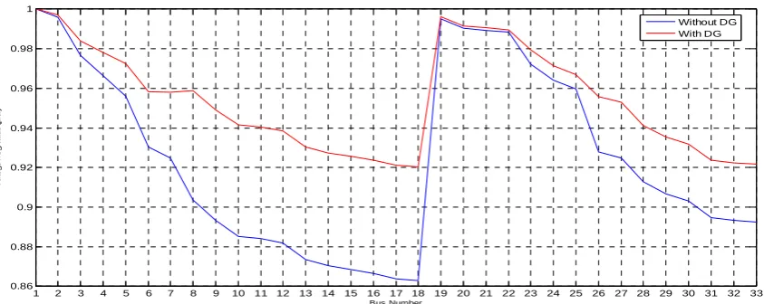
Figure 4 shows voltages at all buses with DG at bus 8 and without DG. The voltage profile was improved.
Figure4:Voltage at all buses with DG at bus8 and without DG
5. Conclusions
Using exact loss formula the size and location of DG unit is found. The DG unit is placed at optimal location which is reducing power loss as well as reactive power loss. The results are tabulated in Table1, Table2, and Table-3.
Table-1 Total active power losses at p.f 0.83
Bus No.
TPL(kw)
Without DG
With DG
%Loss reduction
7 292.47 173.79 40.58
8 292.47 146.22 50.00
9 292.47 167.88 42.82
31 292.47 169.07 42.19
Table-2 Total reactive power losses at p.f 0.83
Bus No.
TQL(KVAR)
Without DG
With DG
%Loss reduction
7 196.07 113.32 42.21
8 196.07 93.84 52.14
9 196.07 107.99 44.92
31 196.07 117.72 39.96
Table-3 Voltages with and without DG at p.f 0.83
Bus No.
Voltage(p.u)
Without DG
With DG
%Voltage Increment
7 0.925 0.958 3.57
8 0.903 0.958 6.11
9 0.893 0.949 6.24
31 0.894 0.924 3.24
1 2 3 4 5 6 7 8 9 10 11 12 13 14 15 16 17 18 19 20 21 22 23 24 25 26 27 28 29 30 31 32 33
0.86 0.88 0.9 0.92 0.94 0.96 0.98 1
Bus Number
Vol
tag
e M
agn
it
u
de (
p.
u.
)
6.References
[1] Duong Quoc Hang,Nadrajah Mithulanathan and R.C.Bansal,”Analytical expressions for DG allocation in primary distribution Networks”,IEEE Trancations on energy conservation,vol.25,No.3,September 2010.
[2] Fernado L.Alvarado.2001.Locational aspects of distributed generation.
[3] Gregery,W.Massey,”Essentials of Distributed generation systems”,Jones&Borlett publishers,Canada,2010
[4] Hasan Hedayati , S.A.Nabaviniaki , Adel Akbarimajd , " A method forplacement of DG units in distribution networks ", IEEE Trans.PowerDelivery , vol 23,no3July 2008.
[5] K.Vinoth kumar and M.P.Selvan,”A Simplified approach for load flow analysis of radial distribution etworks”,International journal of computer and information engg.,Vol.2,April 2008.