Kent Academic Repository
Full text document (pdf)
Copyright & reuse
Content in the Kent Academic Repository is made available for research purposes. Unless otherwise stated all content is protected by copyright and in the absence of an open licence (eg Creative Commons), permissions for further reuse of content should be sought from the publisher, author or other copyright holder.
Versions of research
The version in the Kent Academic Repository may differ from the final published version.
Users are advised to check http://kar.kent.ac.uk for the status of the paper. Users should always cite the published version of record.
Enquiries
For any further enquiries regarding the licence status of this document, please contact: [email protected]
If you believe this document infringes copyright then please contact the KAR admin team with the take-down information provided at http://kar.kent.ac.uk/contact.html
Citation for published version
Song, Yan and Hong, Xinhai and McLoughlin, Ian Vince and Dai, Li-Rong (2016) Image Classification
with CNN-based Fisher Vector Coding. In: IEEE International Conference on Visual Communications
and Image Processing 2016, 27-30 Nov 2016, Chengdu, Sichuan, China. (In press)
DOI
Link to record in KAR
http://kar.kent.ac.uk/57115/
Document Version
Image Classification with CNN-based Fisher Vector
Coding
Yan Song
1, Xinhai Hong
1, Ian McLoughlin
2, Lirong Dai
1 1Department of EEIS, University of Sci. and Tech. of China, Hefei, Anhui, China 2
School of computing, University of Kent, Medway, UK
1{songy,lrdai}@ustc.edu.cn 1[email protected] 2[email protected]
Abstract—Fisher vector coding methods have been demon-strated to be effective for image classification. With the help of convolutional neural networks (CNN), several Fisher vector coding methods have shown state-of-the-art performance by adopting the activations of a single fully-connected layer as region features. These methods generally exploit a diagonal Gaussian mixture model (GMM) to describe the generative process of region features. However, it is difficult to model the complex distribution of high-dimensional feature space with a limited number of Gaussians obtained by unsupervised learning. Simply increasing the number of Gaussians turns out to be inefficient and computationally impractical.
To address this issue, we re-interpret a pre-trained CNN as the probabilistic discriminative model, and present a CNN based Fisher vector coding method, termed CNN-FVC. Specifically, activations of the intermediate fully-connected and output soft-max layers are exploited to derive the posteriors, mean and covariance parameters for Fisher vector coding implicitly. To further improve the efficiency, we convert the pre-trained CNN to a fully convolutional one to extract the region features. Extensive experiments have been conducted on two standard scene benchmarks (i.e. SUN397 and MIT67) to evaluate the effectiveness of the proposed method. Classification accuracies of 60.7% and 82.1% are achieved on the SUN397 and MIT67 benchmarks respectively, outperforming previous state-of-the-art approaches. Furthermore, the method is complementary to GMM-FVC methods, allowing a simple fusion scheme to further improve performance to 61.1% and 83.1% respectively.
Index Terms—Image Classification, Convolutional Neural Net-work, Gaussian Mixture Model, Fisher Vector Coding
I. INTRODUCTION
Over the past few decades, Fisher Vector coding (FVC) and its variants [1], [2], [3] stand out as very effective methods for image classification. FVC was originally derived from the Fisher kernel, which aims to combine the benefit of generative and discriminative approaches for pattern recognition [4]. Generally, the FVC process can be roughly divided into front-end feature extraction and back-end modeling stages. Existing methods mostly employ a diagonal Gaussian mixture model (GMM) as a generative model to characterize the distribution of local features, such as SIFT [5] and HoG [6]. The Fisher vector is then derived from the gradients with respect to the GMM parameters, as detailed in Section II.
Recently, deep convolutional neural networks(CNN) applied to FVC have demonstrated state-of-the-art performance by adopting the activations from a single fully-connected layer as
the image or patch features [7], [8], [9]. However, it is difficult to model the complex distribution of high-dimensional region features using the GMM obtained via unsupervised learning methods. Simply increasing the number of Gaussians has substantial impact on computational complexity and storage. In [8], a generative model with an infinite number of Gaus-sians was used for back-end modeling, which can be further approximated by a sparse coding procedure. However, it is still time-consuming to encode the high-dimensional features. As an alternative, Doersch.et.al.proposed a discriminative mode seeking method to discover visual elements from mid-level regions [10]. In [9], a semantic FVC method was proposed, which uses the outputs of a CNN soft-max layer as patch descriptors, and computes the Fisher vector with GMM in the projected natural parameter space.
Unlike existing FVC methods, we reinterpret the pre-trained CNN as a probabilistic discriminative model, and present a CNN based Fisher vector coding method (CNN-FVC). Specif-ically, a CNN pre-trained on ImageNet [11] is first converted into a fully-convolutional one, with which the feature maps of the intermediate and soft-max layers can be efficiently computed. By using the output soft-max probabilities together with activations of the intermediate feature map, the statistics required for the Fisher vector can be derived, as detailed in Section III. The contributions of this work can be summarized as follows.
• We exploit CNN activations from different layers to cover both the front-end feature extraction and back-end modeling stages in FVC. It is known that there exists a gradual transition from low-level visual features and high-level semantics in deep neural networks trained on natural images [12]. Exploiting information from different layers may help to improve the effectiveness of representation. • We use the pre-trained CNN to classify image patches and consider the class posterior probabilities as locally extracted semantic descriptors. This effectively represents an image as a bag-of-semantics. Compared to the unsu-pervised trained GMM, the CNN posteriors may provide more discriminative and accurate information.
• With a limited number of components, the proposed CNN-FVC method can achieve state-of-the-art perfor-mance on MIT67 and SUN397 scene benchmarks. 978-1-5090-5316-2/16/$31.00 c2016 IEEE VCIP 2016, Nov. 27 – 30, 2016, Chengdu, China
II. GMMBASEDFISHER VECTOR CODING
In this section, we will briefly introduce the GMM based Fisher vector coding (GMM-FVC) method by building on the established setup introduced in [1].
The pre-trained CNN is first converted to a fully convolu-tional one by considering the fully connected layers as the convolutions with kernels that cover their entire regions. This conversion allows us to take input of any size and output cor-responding feature maps. Compared to previous works [7], [8], [9], using the fully convolutional neural network can greatly reduce the computational complexity. In GMM-FVC, the re-gion features are extracted from the feature map corresponding to the 7-th fully-connected layer (FC7). Following [1], PCA projection is first applied to reduce the dimensionality and de-correlate the coefficients of region features.
We assume a K-component diagonal GMM in D -dimensional descriptor space, λ={λk = (πk,µk,σk)}Kk=1,
whereπk ∈[0,1], µk ∈RD and σk ∈RD are the mixture
weight, mean vector and diagonal covariance vectors of the
k-th component respectively. Given a descriptor x, we can write the likelihood function asp(x|λ) =PK
k=1πkg(x;λk), where g(x;λk) denotes a Gaussian. The GMM parameters are obtained on a large training set of descriptors using the expectation-maximization (EM) algorithm to optimize a maximum likelihood criterion.
According to [1], for any descriptor x ∈ RD, we define a vector Ψ(x) = (ψ1(x), ψ2(x), . . . , ψK(x)) ∈ RKD. Each
componentψk(x)is a gradient vector ofp(x|λk)with respect
to theµk.1 ψk(x) = 1 √π k γk(x) x −µk σk (1) where γk(x) is the posterior probability or responsibility of
feature xon Gaussian componentλk,
γk(x) =
πkg(x;λk)
PK
j=1πjg(x;λj)
(2) To represent a imageX={x1,x2, . . . ,xT} withT
descrip-tors, the Fisher vector Ψ(X) can be obtained by average-pooling, Ψ(X) = 1 T T X t=1 Ψ(xt) (3) In practice, we further post-process the Fisher vector using
ˆ
Ψ(X) =sign(Ψ(X))p|Ψ(X)|/pkΨ(X)kL
1 (4)
which computes the signed-square of Fisher vector coefficients followed by normalization. This post-processing has been shown to further improve the effectiveness of Fisher vectors in [1].
1For high-dimensional descriptors, using Ψ(
x) is sufficient for good
performance [9].
III. CNN-BASEDFISHER VECTOR CODING
In this section, we first consider the pre-trained CNN as a probabilistic discriminative model, and show its relationship to conventional GMM. Subsequently, we derive the FVC method using outputs of soft-max and intermediate fully-connected layers.
In the GMM-FVC method, the k-th Gaussian posterior can be conceptually represented as γk(x) = Fλk(x), where Fλk(·) is defined by eqn.(2). Similarly, a pre-trained CNN
that consists of L-layers can be parameterized with θ = {θ1, θ2, . . . , θL}. The actual computation within thel-th layer
has two phases: first, a linear convolution of the inputs. For CNNs, these maps are convolutions of the inputs with learned filter parameters. Afterwards, a non-linear activation function, such as a sigmoid or a ReLU [13], and often a spatial pooling or a sub-sampling operation are applied. The CNN output probabilities can be conceptually represented as
γ(xl) =G
θ(l+1:L)(x
l), wherexlare the activations of thel-th
layer, γ(xl) = (γ1(xl), γ2(xl), . . . , γK(xl)), and Gθ(l+1:L)(·)
represents the linear/nonlinear operations in the CNN layers. The main difference is that the GMM parameters are trained using unsupervised EM, while the CNN parameters are obtained using the cross-entropy criterion with supervision. Furthermore, the CNN structure contains millions of param-eters tuned from large scale datasets, which provides much stronger descriptive and discriminative capability.
Let{xt}T
t=1 be the extracted region descriptors, andγ(xt)
be the output posterior probabilities2 of xt.
As shown in [14] and [1], the 0th-, 1st-, and 2nd-order
Baum-Welch statistics can be computed using feature/posterior pairs from a large-scale training set:(xt, γ(xt))Tt=1.
Nk = T X t=1 γk,t, Fk = T X t=1 γk,txt, Sk = T X t=1 γk,txtxTt (5) With these statistics, the parameter of k-th component λk =
{wk,µk,σk} can then be computed as
wk= Nk T , µk = Fk Nk , σk= Sk Nk − µkµTk (6)
This implicitly represents a diagonal GMM that is derived from the activations of intermediate and output soft-max layers3. Given an imageX, the Fisher vector in eqn. (3) can be rewritten by using the computed statistics.
Ψk(X) = (Fk−Nkµk)/(T√wkσk) (7)
For the ImageNet dataset, there are 1000 classes corresponding to various object classes [11]. In our implementation, we select K(=100) classes according to descending order of their 0th
-order statisticsNk. Similar to in GMM-FVC, the FC7 layer is
used for front-end feature extraction, since it has been proven that the FC7 activations are discriminative and generalizable
2For simplicity, we omit the superscript that indicates activations from the l-th layer
3The multiplication and division of vectors should be understood as
for various image classification tasks [15]. It is worth noting that FC7 and soft-max activations can be computed in a single CNN feed-forward pass, which is more efficient compared to the sparse coding method in [8].
IV. IMPLEMENTATION
We use the excellent MatConvNet toolbox to implement the proposed CNN-FVC method [16]. The pre-trained CNN on large-scale ImageNet [11] is first converted into a full-convolutional one due to its efficiency for region feature ex-traction [17]. Two CNN structures with different complexities (namely AlexNet [18] and VGG16 [19]) are employed as feature extractors. The input images are firstly resized so that their minimum dimension is at least 512, and then fed into the fully convolutional neural network, creating feature maps with about10×15size in different layers. Specifically, the front-end features are extracted from the feature map of the FC7 layer, and the corresponding posteriors are from the output soft-max layer. For the FC7 features, we first reduce the dimension to 512 using PCA. For the soft-max posteriors, as aforementioned, we select 100 classes according to the descending order of{Nk}1000k=1.
Once the features and corresponding posteriors are extract-ed, we encode them using the proposed CNN-FVC method, and generate the image-level representation by average-pooling and normalization. We use libsvm [20] as the SVM solver, and precompute the linear kernels as the inputs. This is because kernel matrix computation actually occupies most of computational time when the feature dimensionality is high. Furthermore, linear kernel computation can be implemented efficiently in parallel.
Table I lists the computational complexities of the feed-forward pass in terms of seconds using the MatConvNet toolbox. All evaluations are conducted on a server with Intel I7-2700k CPU and NVIDIA GTX 980 GPU card installed. From Table I, we can see that VGG16 is computationally heavier than AlexNet. However, the feed-forward pass from the FC7 to soft-max layer, only costs an extra 0.07s in CPU time and 0.01s in GPU time.
TABLE I
THE COMPUTATIONAL COMPLEXITIES OF FEATURE EXTRACTION USING
ALEXNET ANDVGG16.
structures Layer name CPU GPU VGG16 soft-max 1.54s 0.08s FC7 1.50s 0.07s AlexNet soft-max 0.24s 0.02s FC7 0.17s 0.01s
V. EXPERIMENT ANDANALYSIS
We evaluate the proposed CNN-FVC method on two benchmarks: MIT67 [23] and SUN397 [24] datasets. For comparison, we further implement the GMM-FVC method with the FC7 features, as shown in section II. For GMM-FVC, the FC7 features are first reduced to 512-dimensions using PCA, and then GMM-FVC is implemented with a
TABLE II
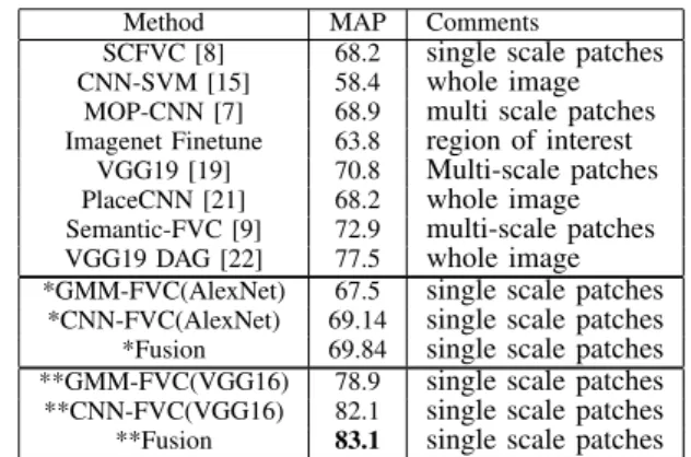
CLASSIFICATION RESULTS ONMIT67DATASET IN TERMS OFMAP(%)
Method MAP Comments
SCFVC [8] 68.2 single scale patches
CNN-SVM [15] 58.4 whole image
MOP-CNN [7] 68.9 multi scale patches
Imagenet Finetune 63.8 region of interest
VGG19 [19] 70.8 Multi-scale patches
PlaceCNN [21] 68.2 whole image
Semantic-FVC [9] 72.9 multi-scale patches
VGG19 DAG [22] 77.5 whole image
*GMM-FVC(AlexNet) 67.5 single scale patches
*CNN-FVC(AlexNet) 69.14 single scale patches
*Fusion 69.84 single scale patches
**GMM-FVC(VGG16) 78.9 single scale patches
**CNN-FVC(VGG16) 82.1 single scale patches
**Fusion 83.1 single scale patches
100-component mixture using the public vl feat toolbox [25].
Experiments on MIT67
The MIT67 dataset contains 6700 images over 67 indoor scene categories, with 100 image in each category. This dataset is quite challenging since most scenes are collections of objects organized in a highly variable layout, with some subtle cross-category differences.
We use the standard training/test split which consists of 80 training and 20 test images for fair comparison. The experimental results are shown in Table II. Furthermore, we compare the classification accuracy with previous works [8], [7], [15], [19], [21]. Firstly, we can see that the proposed CNN-FV method outperform the GMM-FV by 1.5%-3% for AlexNet and VGG16 respectively.
With AlexNet, the best performance is 72.9%, which is achieved by using semantic FVC with multi-scale patch fea-tures. It is worth noting that our proposed CNN-FVC could be easily extended to the multi-scale case, but this is left for future work. Compared to the sparse coding based Fisher vector (SCFVC) method [8], the GMM-FVC(AlexNet) with similar settings performs slightly worse, which is consistent with their conclusion. However, the proposed CNN-FVC can outperform SCFVC by 1% absolutely. This validates the idea
TABLE III
CLASSIFICATION RESULTS ONSUN397DATASET IN TERMS OFMAP(%)
Method MAP Comments
MOP-CNN [7] 52.0 multi scale patches
Decaf[26] 40.9 whole image
Semantic-FVC [9] 54.4 multi-scale patches
PlaceCNN [21] 54.3 whole image
VGG19 [19] 51.9 Multi-scale patches
Deep-19 DAG [22] 56.2 Multi-scale features
*CNN-FVC(AlexNet) 52.0 single scale patches
*GMM-FVC(AlexNet) 49.0 single scale patches
*Fusion 52.8 single scale patches
**GMM-FVC(VGG16) 58.2 single scale patches
**CNN-FVC(VGG16) 60.8 single scale patches
**Fusion 61.1 single scale patches
that using the features extracted from different layers may help to improve classification performance. The PlaceCNN [21]
method learns an AlexNet directly on a 2 million place dataset [21]. On MIT67, the classification accuracy is about 68.2%, outperforming the 63.8% Imagenet fine-tuning method with the same CNN structure. It would be interesting to try the CNN-FVC method using PlaceCNN in future.
With a more complex VGG16 structure, GMM-FVC achieves 78.9%, outperforming the previously reported state-of-the-art, such as 77.5% of the VGG19 DAG method that uses activations from multiple layers [22]. However, the features extracted at image-level may lack geometric invariance, which limits their robustness for scene classification. The VGG19 [19] method extracts the FC7 activations from multi-scale regions, but it uses a simple average-pooling for final image representation to achieve an accuracy of 70.8%. The result for the proposed CNN-FV is 82.1%, which is particularly impressive compared to the results of GMM-FV (78.9%) and VGG19-DAG (77.5%).
Experiments on SUN397
SUN397 [24] is a large scale scene recognition dataset with about 100K images spanning 397 categories. The evaluation protocol involves publicly available train-test splits, each with 50 training and 50 test images. Table III reports our results on the SUN397 dataset. From the results, we can see that CNN-FVC works consistently better than GMM-FVC, with about 2%-3% performance gap for both AlexNet and VGG16 CNN structures. Among AlexNet CNN structures, the best performance for SUN397 is achieved by Semantic-FVC [9] using multi-scale features, which is slightly better than PlaceC-NN [21]. For the VGG16 CPlaceC-NN structure, the proposed CPlaceC-NN- CNN-FVC method achieves an accuracy of 60.8%, outperforming the previous best result of 56.2% by a significant margin.
Furthermore, for MIT67 and SUN397, the fusion CNN-FVC and GMM-FVC systems can improve the accuracy to 61.1%. In comparison, simply increasing component numbers from 100 to 200 has inly a slight performance improvement in our experiments.
VI. CONCLUSION
In this paper, we presented a CNN-FVC method by treating a pre-trained CNN as the probabilistic discriminative model. More specifically, activations from an intermediate layer (FC7) and the output soft-max layer are used for both front-end fea-ture extraction and back-end modeling stages in conventional FVC methods. These activations can be efficiently obtained through a single feed-forward pass. Compared to GMM-FVC, the CNN-FVC method can effectively describe the complex distribution of the high-dimensional feature space with the help of the CNN structure. The experimental results on two standard scene benchmarks (i.e. SUN397 and MIT67) validate the effectiveness of the proposed CNN-FVC method. Classi-fication accuracies of 60.7% and 82.1% can be achieved on SUN397 and MIT67 benchmarks respectively, outperforming previously reported state-of-the-art results.
ACKNOWLEDGMENT
The authors would like to acknowledge the support of National Natural Science Foundation of China grant no. 61172158.
REFERENCES
[1] J. Sanchez, F. Perronnin, T. Mensink, and J. J. Verbeek, “Image classification with the Fisher vector: Theory and practice.”International Journal of Computer Vision, vol. 105, no. 3, pp. 222–245, 2013. [2] X. Zhou, K. Yu, T. Zhang, T. S. Huang, and T. S. Huang, “Image
classification using super-vector coding of local image descriptors.” in
Proc. of ECCV, 2010, pp. 141–154.
[3] H. Jegou, M. Douze, C. Schmid, and P. P1717rez, “Aggregating local descriptors into a compact image representation.” in Proc. of CVPR, 2010, pp. 3304–3311.
[4] T. Jaakkola and D. Haussler, “Exploiting generative models in discrim-inative classifiers,” inProc. of NIPs, 1998, pp. 487–493.
[5] D. G. Lowe, “Distinctive image features from scale-invariant keypoints,”
International Journal of Computer Vision, vol. 60, no. 2, pp. 91–110, 2004.
[6] N. Dalal and B. Triggs, “Histograms of oriented gradients for human detection,” inProc. of CVPR, 2005, pp. 886–893.
[7] Y. Gong, L. Wang, and R. Guo, “Multi-scale orderless pooling of deep convolutional activation features,” inProc. of ECCV, 2014, pp. 392–407. [8] L. Liu, C. Shen, L. Wang, A. van den Hengel, and C. Wang, “Encoding high dimensional local features by sparse coding based Fisher vectors,” inProc. of NIPs, 2014, pp. 1143–1151.
[9] M. Dixit, S. Chen, D. Gao, N. Rasiwasia, and N. Vasconcelos, “Scene classification with semantic Fisher vector,” inProc. of CVPR, 2015. [10] C. Doersch, A. Gupta, and A. A. Efros, “Mid-level visual element
discovery as discriminative mode seeking,” inProc. of NIPS, 2013, pp. 494–502.
[11] J. Deng, W. Dong, R. Socher, L. Li, K. Li, and F. Li, “Imagenet: A large-scale hierarchical image database,” inProc. of CVPR, 2009, pp. 248–255.
[12] J. Yosinski, J. Clune, Y. Bengio, and H. Lipson, “How transferable are features in deep neural networks?.” inProc. of NIPs, 2014.
[13] V. Nair and G. E. Hinton, “Rectified linear units improve restricted Boltzmann machines,” inProc. of ICML, 2010.
[14] C. M. Bishop,Pattern Recognition and Machine Learning. Springer, 2006.
[15] A. S. Razavian, H. Azizpour, J. Sullivan, and S. Carlsson, “CNN features off-the-shelf: an astounding baseline for recognition,”CoRR, vol. abs/1403.6382, 2014.
[16] A. Vedaldi and K. Lenc, “Matconvnet – convolutional neural networks for MATLAB,” vol. abs/1412.4564, 2014.
[17] J. Long, E. Shelhamer, and T. Darrel, “Fully convolutional network for semantic segmentation,” 2015.
[18] A. Krizhevsky, I. Sutskever, and G. E. Hinton, “Imagenet classification with deep convolutional neural networks,” inProc. of NIPs, 2012, pp. 1106–1114.
[19] K. Simonyan and A. Zisserman, “Very deep convolutional networks for large-scale image recognition,” 2015.
[20] C.-C. Chang and C.-J. Lin, “Libsvm: A library for support vector machines,”ACM Transactions on Intelligent Systems and Technology, 2011.
[21] R. Arandjelovic, “Learning deep features for scene recognition using place database,” inProc. of NIPS, 2014.
[22] S. Yang and D. Ramanan, “Multi-scale recognition with DAG-NN,” in
Proc. of ICCV, 2015.
[23] A. Quattoni and A. Torralba, “Recognizing indoor scenes,” inProc. of CVPR, 2009, pp. 413–420.
[24] J. Xiao, J. Hays, K. A. Ehinger, A. Oliva, and A. Torralba, “SUN database: Large-scale scene recognition from abbey to zoo,” 2010, pp. 3485–3492.
[25] A. Vedaldi and B. Fulkerson, “VLFeat: An open and portable library of computer vision algorithms,” ”VLFeat.org. Available: http://www.vlfeat.org/”, Accessed 2014 June 30, 2008.
[26] J. Donahue, Y. Jia, O. Vinyals, J. Hoffman, E. T. N. Zhang, and T. Darrell, “Decaf: A deep convolutional activation feature for generic visual recognition,” inProc. of CVPR 2014, 2014.