AN ADAPTIVE GRID-BASED METHOD
FOR CLUSTERING
MULTI-DIMENSIONAL ONLINE DATA
STREAMS
Toktam Dehghani
Department of Computer Engineering, Ferdowsi University Mashhad, Mashhad, Khorasan Razavi, Iran
[email protected] http://toktamdehghani.com
Mahmoud Naghibzadeh
Department of Computer Engineering, Ferdowsi University Mashhad, Mashhad, Khorasan Razavi, Iran
[email protected] http://profsite.um.ac.ir/~naghibzadeh/
Mohamadreza Afsharisaleh
Department of Engineering, Islamic Azad University, Mashhad, Khorasan Razavi, Iran, [email protected]
Abstract:
Clustering is an important task in mining the evolving data streams. A lot of data streams are high dimensional in nature. Clustering in the high dimensional data space is a complex problem, which is inherently more complex for data streams. Most data stream clustering methods are not capable of dealing with high dimensional data streams; therefore they sacrifice the accuracy of clusters. In order to solve this problem we proposed an adaptive grid -based clustering method. Our focus is on providing up-to-date arbitrary shaped clusters along with improving the processing time and bounding the amount of the memory u sage. In our method (B+C tree), a structure called “B+cell tree” is used to keep the recent information of a data stream. In order to reduce the complexity of the clustering, a structure called “cluster tree” is proposed to maintain multi dimensional clusters. A Cluster tree yields high quality clusters by keeping the boundaries of clusters in a semi -optimal way. Cluster tree captures the dynamic changes of data streams and adjusts the clusters. Our performance study over a number of real and synthetic data streams demonstrates the scalability of algorithm on the number of dimensions and data without sacrificing the accuracy of identified clusters.
Keywords: data streams; data mining; clustering; grid-based clustering; high dimensional data streams. 1. Introduction
During the recent years, data streams have attracted attention in different applications of computer science, such as customer click streams, multimedia data, sensor data, network monitoring, telecommunication system, stock markets. A data stream is defined as a massive unbounded sequence of data elements continuously generated at a rapid rate [Park and Lee (2007)]. Management and processing of these online rapid unbounded streams raises new challenges because the traditional algorithms are usually not feasible to perform operations [Beringer and Hüllermeier (2003)]. Online data stream processing should satisfy the following requirements [Park and Lee (2007)]:
1. Each data element should be examined at must once to analyze a data stream.
2. Memory usage for data stream analysis should be confined finitely although new elements are continuously generated in a data stream.
3. Newly generated data elements should be processed as fast as possible to produce the up-to-date analysis result of a data stream.
clustering of multi dimensional data streams. Our focus is on providing up-to-date arbitrarily shaped clusters along with processing as fast as possible and bounding the amount of memory space used to maintain information.
The remainder of the paper is organized as follows: section 2 provides some background information on data streams clustering algorithms. In section 3, a method for clustering data streams is proposed. In section 4, several experiment results are analyzed to evaluate the performance of the proposed method.
2. Related work
Clustering is one of the major data mining categories and it groups a set of data into classes called cluster. Clustering techniques are categorized into several different approaches. Partitioning, hierarchical, density-based, grid-based and model-based [Park and Lee (2007)][Guha et al. (2003)]. There are several clustering algorithms for data streams that use different approaches. In the following, data streams clustering algorithms such as STREAM [Guha et al. (2003)], CluStream [Agrawal et al. (2003)], HPStream [Agrawal et al. (2004)], EStream [Thanawin et al. (2007)], DenStream [Cao et al. (2006)], DStream [Chen and Yu (2007)], cell tree [Park and Lee (2007)], and CS tree [Jae, et al. (2009)]are discussed.
In [Guha et al. (2003)], STREAM and LSEARCH algorithms are proposed to find the clusters of the continuously generated data elements over a data stream [Park and Lee (2007)] [Muthukrishnan (2003)]. It regards a data stream as a sequence of stream chunks. A stream chunk is a set of consecutive generated data elements that fits in the main memory. For each chunk, STREAM clusters its elements and retains the weighted cluster centers. The centers are weighted according to the number of elements attracted to them. Then, the weighted centers are retained for each examined chunk so far, to obtain a set of weighted centers for entire stream. STREAM uses LSEARCH which is a 0(1)–approximate k-means algorithm for clustering of the chunks and weighted centers. Although this algorithm makes a single pass over a data stream and uses small spacey, when the number of clusters is not known in advance, the LSEARCH routine should be iteratively performed until the quality of clusters is maximized, which makes it not directly applicable to data stream [Park and Lee (2007)] and like other partitioning approach, STREAM is incapable of revealing clusters of arbitrary shapes and detecting noise and outliers [Chen and Yu (2007)].
A hierarchical algorithm called CluStream [Agrawal et al. (2003)]is proposed for the clustering of evolving data streams. It divides the clustering process into the on-line and off-line components. The on-line component computes and stores statistics about the data stream using micro clusters. The information of a micro cluster is represented by a cluster feature vector which is similar to the cluster feature vector of BIRCH. The on-line micro cluster processing is divided into two phases: statistical data collection and updating of micro clusters. In the first phase, the totals of micro clusters are maintained. The predefined number of micro clustering is determined by the available space of main memory. In the second phase, micro clusters are updated when a new data element is processed. If the new data element falls within the boundary of an existing cluster, the feature vector of the micro cluster is updated by the new data element; otherwise, a new cluster with unique ID is created for the new data element. In this case, the number of micro clusters becomes larger than the predefined one; the nearest two micro clusters are merged into the one micro cluster or the oldest micro clusters are deleted. However the CluStream uses the predefined constant number of micro clusters which is especially risky for the evolving data stream [Chen and Yu (2007)]. This algorithm is not suitable for finding clusters over online data stream due to its offline components. To cluster evolving data stream based on both historical and current stream data, the snapshots of a set of micro clusters are stored at different levels of granularity, so more information maintain for more recent events as opposed to older events. In the off-line component, the macro clusters of CluStream are generated by executing the k-means algorithm for the accumulated snapshots of micro cluster. This component can perform user-directed macro clustering as cluster evolution analysis. To allow a user to explore the stream clusters over a specified time period 'h', the two snapshots of the micro cluster at the times 'tc' and 'tc-h' are compared. The k-means algorithm is executed on the subtracted cluster feature vectors. To analyze the evolution of micro cluster in the period 'h' ids of clusters in two snapshots are compared and the added, deleted or retained clusters are identified. CluStream yields high quality clusters and it maintains scalability in term of stream size. However, this algorithm is not suitable for finding clusters over a one-line data stream due to its off-line component.
essential to design methods which efficiently adjust to the progression of streams. HPStream assigns to each cluster a bit-vector which corresponds to the relevant set of dimensions of data of the stream. Each element in this vector has 0-1 value according to whether or not a given dimension is included in that cluster. As the algorithm progress, this bit vector updates in order to reflect the changing set of dimensions. HPStream uses a fading cluster structure to be able to adjust the clusters in a flexible way. Fading cluster structure captures a sufficient number of statistics, so it is possible to compute key characteristics of the clusters. A function called fading function is defined which is a monotonic decreasing one and its values lies in the range (0,1). This function is exponential and gradually discounts the history of past behavior. HPStream is incrementally updatable and scalable on both the number of dimensions and size of the data stream and in comparisons with STREAM and CluStream, it achieves better clustering quality for high dimensional data [Agrawal et al. (2003)]. Since the characteristics of the data in streams evolve over time, various types of evolution should be supported by algorithms. In order to improve existing stream clustering algorithms, EStream [Thanawin et al. (2007)] was presented. EStream classifies evolution of clusters into five categories: appearance, disappearance, self evolution, merge and split. In this technique, incoming data, based on similarity score, may be assigned to an active cluster or be classified as on isolated. Eventually, if the region becomes dense, a new cluster appears. Existing clusters that contain only old data are faded, and ultimately disappear. By analyzing histograms, clusters can be split. Also, this algorithm checks every pair of cluster and merges the overlapping ones. If the number of clusters exceeds the defined limit, the algorithm merges the closest pairs. EStream improved stream clustering algorithms by supporting data evolutions and presenting a new suitable cluster representation and a distance function. However, EStream requires a limit on the number of clusters that may cause incorrect clustering. This algorithm needs a lot of data accommodated for appearance of initial clusters and detecting some evolutions such as merge. EStream exhibit linear runtime in the number of dimensions but polynomial one in the number of clusters due to the merging procedure.
Previous proposed streaming algorithms produce spherical clusters. A density-based algorithm called DenStream [Cao et al. (2006)] was introduced to overcome these drawbacks. This algorithm can be divided into two parts: online part for maintaining micro cluster and offline part for generating the final clusters. In order to summarize the clusters with arbitrary shapes, the micro cluster synopsis is designed by a set of micro clusters. Clusters are found by applying DBSCAN in offline part. In addition to distinguishing potential clusters and outliers, DenStream stores them as micro clusters in an online way and separates their processing and memory space. For each new data if it's far from all potential and outliers-micro clusters, it creates a new outlier-micro cluster. An outlier-micro cluster whose weight is more than the threshold will be converted into a potential micro cluster. To limit memory consumption, DenStream uses a pruning strategy which provides opportunity for the growth of new clusters while promptly getting rid of outliers. So, in this algorithm no assumption on the number of clusters is needed. DenStream achieves consistently high clustering quality, but the some overall density for the absolute parameters making the result of clustering sensitive to parameter values. This algorithm cannot distinguish clusters which have different levels of density.
DStream [Chen and Yu (2007)] is a density and grid-based algorithm like DenStream algorithms. DStream also tries to resolve incompetent to find clusters of arbitrary shapes. The difference is that it’s a grid based algorithm using the density grid structure. The algorithm uses an online component which maps each input data record into a grid cell and an offline component which computes the grid's density and clusters the grids based on their density. In online component, the space is partitioned into fine grids and new data records are mapped into the corresponding grid. The algorithm adapts a density decaying technique to capture the dynamic changes of a data stream. The offline component dynamically adjusts the cluster in every gap time. A grid cluster is a connected grid group which has higher density than the surrounding grids. Grids that are under consideration for clustering analysis are maintained in a grid –list. The grid list is implemented as a hash table to allow fast access and update. Further, a technique is developed to detect and remove sporadic grids mapped to by outliers. In this algorithm, sporadic grids that have previously received many data but the density is reduced by the effect of decay factor are not be removed and marked as sporadic because they may become dense in the future. During clustering algorithm, considering unsporadic grids in the grids list instead of the possible grids saves computing time, and space of the system. However, DStream algorithm does not perform well on the high dimensional data streams due to requiring very large number of grids.
obtained. predefine data elem dimensio space. A Among th are corre estimated sacrificin Due to o following be scann because o grid cell discovere streams, dimensio tries to fi not preci and this number o Fig. 1(a) (c1,c2) an to make only thre dimensio tree finds
3. The p In this se following
3. 1 fund
A data st ek. . . } a dimensio
We note applicatio stream. D generated updating
3. 2. A fa
To find c should b dividing explore c dynamica the cell i
. The result ed sequence o ments in the onal clusters C A node corresp he leaf nodes esponding to t d by a data ng the accurac ur study, ther gs are the CS ned in a sequ
of the defined s, few numbe ed. Third, in th in the first onal clusters a find the real c ise. The result may lead to of clusters mak
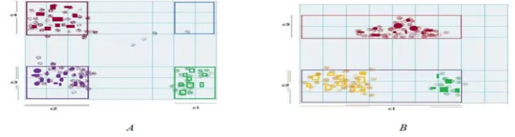
) shows a tw nd in the y dim the final clust ee clusters. Fig on, in the x dim
s three cluster
proposed algo ection, we pres g the proposed
damental conc
tream for a d-d arriving at tim ons, denoted b
e that since ons naturally Due to this re d data elemen the distributio
fading structu
clusters over a e carefully m a multi dime clusters in hig
ally partitionin in the grid. Th
of this match of dimensions.
space over t CS tree is use ponding to a whose depth the final clust distribution s cy of identified
re are some pr tree's problem ential manner d partition thre
ers of the da his algorithm, step one–dim re combined b clusters by fin
ts show that t overlap of th kes the proble wo dimensiona mension there ters. So, CS tr g. 1(b) shows mension there s in this data s
orithm (B+C sent the funda d algorithm is
cepts
dimensional d me stamps {T by:
a data stream impose a limi eason, it is ess nts of a data s
on statistics o
ure for monito
a data stream a monitored. A c ensional spac gher dimension
ng the data sp he number of
hing is repres The support the total num ed. A k-depth
dense multi d are the same a ters. For impr synopsis. This
d clusters. roblems in the ms: First, for e
r to find the eshold, in the r ata elements b , in order to re mensional clus by CS tree and nding a freque
the number of he clusters (o em more obvio al data space, e are two clus ree finds four a two dimens e is one cluste space due to th
Fig. 1) an exa
tree) amental conce
described.
data space N=N 1…. Tk …. }
e m is a massi ited memory c sential to use tream. In the f data element
oring the distr
accurately, the common way e into the fin ns. In order to pace into a nu points inside
sented by a of a rectangu mber of data h node in CS dimensional r as the dimens roving the clu s algorithm i
e CS tree met each data elem
related interv recursive proc belong to the educe the com sters in each d make the m ently co-occur f multi-dimen occultation). I ous. Also, upd , in this data sters (c3,c4). I r clusters in th sional data spa er (c1) and in t the overlappin
ample of clusterin
epts of the grid
N1 ×. . . ×Nd, Each data po
e , … , e ive unbounde constraint, it i
a scalable m next section, ts.
ribution statis
e distribution to find clust nite intervals o monitor the umber of the cell can b
list of match lar space is de elements gen tree is corres rectangle spac sionality of the ustering, the p is scalable on
thod that can ment, a single val which is cedure of part e final cluster mplexity of the dimension a multi-dimension
rred set of on nsional cluster
Increasing the dating of mult space in the In CS tree, on his data space ace, in this da the y dimensi ng of clusters,
ng with CS tree
d which is ma
Consists of a oint ei is a mu
.
ed sequence s impossible t method to mon we will discu
stic of data ele
statistics of c ters and high-(cells) in eac distribution o overlapping r be used to de
hed cluster id efined by the r nerated so fa sponding to a
ce is allowed e data stream precise range n the number
be solved to g linked list in a time consum itioning the gr rs and many e clustering of are traced, th nal clusters. A e-dimension c rs and their ou e density of t
ti dimension c x dimension e-dimensional e due to the no ta space after on there are tw however there
inly based on
set of d-dime ulti-dimension
of data elem to maintain all nitor the distri
uss the structu
ements
ontinuously g -density region ch dimension,
f data, a histo egions and th termine the d
dentifiers orde ration of the n ar. In order t
k-dimension d to have a ch and have high of each final r of dimensio
gain better re each dimensi uming process rid cells to fin small cluster f high dimens hen a sequenc
Although, the clusters, this m utliers are no the data spac clusters is not there are tw al clusters are oise, however projecting da wo clusters (c re are only two
CS tree and t
ensional recor nal record con
ments and da ll the elements ibution of con ure for mainta
generated data ons in the data
, which are m ogram is const hen mapping t density (count)
ered by a number of to find
d-rectangle hild node. h supports cluster is ons while sults. The on should s. Second, nd the unit
rs are not ional data ce of one
algorithm method is t accurate e and the precise. o clusters combined r there are ata in each c2,c3). CS o clusters.
then in the
rds { e1. . . ntaining d
ata stream s of a data ntinuously aining and
and deviation of the data elements of the cell. Clustering patterns embedded in a data stream usually change as times goes by. In order to keep only the recent information of a data stream, the weight of information represented by each data element should be differentiated according to the generated time of the data element. To identify the recent change of data elements, a fading factor is used. A fading factor determines how fast the effect of old information is faded away. According to [Javitz and Valdes (1994)], the weight of information represented by a data element generated in a data stream can be decayed based on the decay rate (
τ
). The recent distribution statistics of a cell are defined as follows [Park and Lee (2007)]:)
1(
ct cv τt‐v 1
)
2(
µt µv
cv τt‐v et
ct
)
3(
δt cv
ct δv 2 τ
t‐v µ
v 2
et 2
ct ‐ µ t 2
In these equations,
τ
, Ct, µ t, δ denote as follows:
τ
is the decay rate based on the model representation in [Javitz and Valdes (1994)]. Ct is the decayed count of data elements in the cell until 't'.
µ
tis the decayed average of the data elements in the cell until 't'.
δis the standard deviation the data elements in the cell until 't'.
v is the latest update time of the cell.
3. 3. Parameters of the proposed algorithm
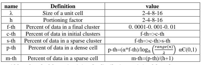
In our algorithm several parameters are used to manage clustering of data streams. The parameters are summarized in table 1.
Table 1: Clustering parameters
name Definition value
λ Size of a unit cell 2-4-8-16
h Portioning factor 2-4-8-16
f-th Percent of data in a final cluster 0. 0001-0. 001-0. 01 c-th Percent of data in initial clusters f-th=>c-th s-th Percent of data in a sparse cluster f-th=>c-th>s-th
p-th Percent of data in a dense cell p-th=(α*f-th)/log αЄ(0,1)
m-th Percent of data in a sparse cell m-th=(p-th)/(h+1)
3. 4. Adaptive grid-based method for maintaining the distribution statistic of data elements
In this paper, adaptive grid –based clustering is used for clustering of data elements in data streams. Grid-based clustering algorithms first cover the data space with grid cells. Statistical distribution is collected for all the data objects. Regions which have more points than a specified threshold are identified as dense. Dense regions that are adjacent to each other are merged to find the embedded clusters.
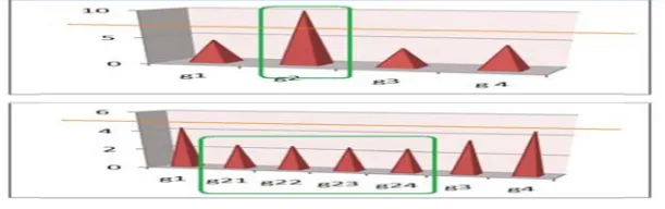
Given the current data stream Dt for each one-dimensional data space N, distribution statistics of the corresponding cell, is updated. When the cell is dense enough, it is partitioned into smaller equal-size cells. Since such partitioning can be performed recursively in dense regions of the data space, the distribution statistics of these regions become more accurate. The current density of a cell is the ratio of the number of these data elements that are inside the interval of the cell over the total number of data elements. When the current density of a cell (g) is greater than or equal to partitioning threshold (p-th). It is partitioned into h (a predefined partitioning factor) smaller equal-size cells. The distribution statistics of new cells gi (1<= i <= h) are initialized by the normal distribution of as follows [Park and Lee (2007)]:
)
4(
φ x 1
g. δ √2πe
.µ .
)
5(
g . .
.
In these e
In fig. 2 t g14). This part smallest of data el was dens By merg consider current d cell over such a ce
3. 5. B+c
In order "B+cell" t a faster fi retrieving defined a
In B+cell
equations g . g . is the g . is the g . δis the the cell g2 is j
titioning proc cell in the dat lements in a d se in the past.
ging these spa a decay rate f density of a ce the total num ell is merged w
cell tree
to manage th tree is propos finding and up g the distribut as follows:
Each node Id of each relationshi All leaves
tree, two kind Non-leaf n Leaf node structure fo
g .
g . δ
.
, g . and g e count of data e average of da e standard dev
ust becoming
edure can be ta space and in data stream ca
Fig. 2
arse cells, unn for reducing w ell is low, the mber of data e with a set of h
he dynamically sed. B+cell tree pdating of the
tion statistic o
e will contain a h cell is defin
ip according to appear in the
ds of nodes ar nodes: This kin es: This kind for storing dist
.
. .
g . δ denote a a elements in g
ata elements i iation of data g dense in the
recursively in nterval size of an be changed
2) A dense cell po
necessary cell weight of cells ratio of the d elements becom
-1 sparse neig
y varied conf e(based on B+ distribution st f neighbors' c
a number of c ned by the be o their ids.
same level, an
re defined (Fig nd of node inc of node incl tribution statis
F
.
as follows: gi until 't'. in gi until 't'.
elements in g t-th turn and i
nvoked until f every unit ce d as time goes
ortioning process
ls are elimina s which are n decayed numb
mes less than ghbor cells.
figuration of c +
tree) provide tatistics of the cell in the mer
cells vary betw eginning of it
and carrying th
g. 3): cludes a list o ludes a list o stic of a cell, c
Fig. 3) B+cell tre
gi until 't'. is partitioned
a unit cell is ell is the same by, a specific
s [Park and Lee (2
ated and the m ot updated in ber of these da n or equal to p
cells in the en es of random a e cells, also m rging and the c
ween M/2 and ts range. Amo
he distribution
f cell's ids and f cell's ids an called cell’s in
ee
into smaller d
found. A uni e as λ. Since th c cell may bec
2007)]
memory usag the recent tur ata that are in predefined me
ntire range of access to the c makes a sequen clustering pro
m (except roo ong the cells
n statistic of th
d a list of poin nd a list of p nfo-box.
)
6(
)
7(
disjoint cells (
it cell is defin he distribution come sparse a
ge can be red rns. For a cell nside the inter erging thresho
f data space e cells in order t ntial access po oducers. A B+c
ot).
exists a total
he cell.
nters to its chi pointers to th
(g11 g12 g13
ned as the n statistics although it
duced. We l, when he rval of the old (m-th),
efficiently, to prepare ossible for cell tree is
l ordering
Theorem 1: Given a partitioning factor h for a data set of a one-dimensional data space N, the minimum number of recursive partitioning operation needs to produce a unit cell is log [Agrawal et al. (2005)]. Theorem 2: In a B+ cell tree, if n is the number of data elements and m is the maximum number of children a node can have, the average time complexity of searching, insertion and deleting will be log n [Mehta and Sahni (2004)].
Assume the total number of cells in B+cell tree in one dimensional space is and the maximum number of children that a node can have is h, then according to the theorem 1 and 2, the average height of a B+cell tree is log range N /λ. The average time complexity of operations will be under the minimum number of the recursive partitioning operation needs to produce a unit cell.
Definition 1: insert procedure
(1) For each new cell, perform a search to determine related leaf node. Record the path in a stack. (2) Insert id of new cells to the related node and the pointer to the cell's info-box.
(3) If the node is full (more than m cells in a node),
(i) Allocate new the leaf and move half of the node's cells to new cell. (ii) Update the extra pointer of the node, its neighbors and the new node. (iii) Insert the smallest id of the new leaf into the parent.
(4) If the parent is full, split it.
(i) Add the middle id to the parent node.
(ii) Repeat until a parent is found that does not need to split.
(5) If the root splits, create a new root which has one cell and two pointers.
Definition 2: partitioning procedure
If the number of these data elements that are inside the interval of a cell over the total number of data elements is greater than equal to partitioning threshold (P-th), the cell is partitioned as follows:
(1) Split range of the cell into the h number of smaller equal cell. Create h-1 new ids. (2) Initialize the distribution statistics of new cells.
(3) Assign a value between 0 to h-1, to each small cell according to their orders.
(4) If a small cell has the same id as its parent cell, replace the parent cell with the small cell. (5) Else insert the (h-1) small cells into the B+cell tree.
Definition 3: removing procedure
To merge the neighboring cells, each cell is removed as follows:
(1) Start at root, find leaf node where the cell belongs. Remove the cell.
(2) If the cell's id is the smallest in the node, update parent with the second smallest id in the cell. (3) If a leaf node is more than half-full, done!
(4) If a leaf node cells less than it should,
(5) If sum of number of cells in it and one of its adjacent nodes is more than m/2 Try to re-distribute, borrowing from the adjacent node.
Else
Merge a node which sum of number of cells in it and other adjacent node is less than m. The node with bigger id must be deleted.
(6) Merge could propagate to root, decreasing height.
Definition 4: Merging procedure
In partitioning procedure a value between 0 to h-1 is assigned to each new cell. This value shows the place of the new cell in the range of the parent cell; also it helps to recognize cells that were partitioned together. In order to find the sparse cells, leaf nodes of the tree are scanned. In B+cell tree, some of the neighboring cells can be in the other leaf node. Processing of these cell is available by the extra pointer references the nearest neighbor node in the tree. According to the assigned value of the cell, the direction of processing is determined:
(1) If the value is equal to zero, the (h-1) nodes in the right direction will be processed. (2) If the value is equal to h-1, the (h-1) nodes in the left direction will be processed. (3) Otherwise both directions will be processed.
(4) Distribution statistics of all cells are merged.
(5) Except the cell with an id equal to zero, the entire cell's ids are stored in a stack.
(6) If the entire neighbor's of a sparse cell are sparse, they will be merged and replaced by a cell with the smaller id. Other cells are popped from the stack and removed.
We prese of "B+cel
3. 6. Clu
In this tr sequence dimensio (Ck). For Clusters dimensio shows a combines
3. 7. mu
For each dimensio monitors Initially, For the c
Bi,j
Chi
(1) If |B
For (2) If B (i) If (ii) If (3) If B (i) In (ii) Se
ent a "cluster ll tree" and "c
uster tree (C tr
ree, for each es. Based on d onal clusters. E r a cluster in cl
Count: the co Lee (2007)].
v is the last up Cluster's inter real boundari Child []are P dimensional c
interface is a onal cluster is
cluster is cov s the neighbor
ulti-dimension
h new data el on sequence,
the list and it
Bi,j: A corresp
|Bi,j |: Range o
Count (Bi,j): T
Count (ci-1): T
Dt: The total
the root of th orresponding j is dense enou
ild z is sparse Bi,j | < λ then r each child of Bi,j is not dens f childz does n f childz is spar Bi,j is dense an nsert new child end the new c
tree" for com luster tree" m
ree)
data elements dense cells of
Each node in luster tree, the ount of data de
pdate time of rface is a dev es.
Pointers to th clusters.
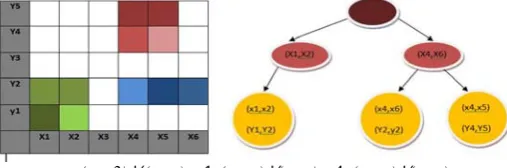
a structure for a set of k-dim vered with 3 h
r hyper-cubes
<(x1,
nal clusters
lement, the c the beginning ts adjacent clu
ponding cell to of j-th cell of i The number of The number of number of dat
he tree is assum cell in each d ugh to be a clu
,
| |
enough to rem
| |
the clustering f the parent clu se,
not exist, then rse, delete chil nd childz does d (cluster) if t child as the par
mposing n-dim makes "B+C tre
s, cells of the f one dimensio
the k-th dept e following fe ements in the
the cluster. eloped structu
he children o
r maintaining mensional hyp hyper cubes. T
.
, x2) ⋁ (x1,y2)> ⋀
Fig.
corresponding g and the end usters to updat
o the new data i-th dimension f data element f data element ta elements un
med as the par dimension the
uster, if
moved from cl g condition is i uster, if in the
stop clusterin ldz and stop c s not exist,
he parent clus rent cluster fo
mensional clus ee".
e one dimensi onal space, on th of a cluster eatures are ma
Ck. Count is
1
ure for mainta
of a cluster.
g the boundari percubes that The proposed
⋀<(x4, x6) ⋁(y2,y2)
4) Clustering inte
g cell, in each d of updated te the result. C
a element in i n
t in the j-th ce t in the paren ntil 't'.
rent cluster an following con
(9)
lusters, if (10) invalid and th e i-th dimensio
ng! clustering!
ster is dense. or next dimens
sters from one
ional spaces a ne-dimension r tree is corre aintained:
calculated acc
aining the bou
Children of
ies of a k-dim covers all th method scans
)> ⋀<(x4, x5) ⋁(y
erface
h-dimensiona cells are ins Clustering is b
-th dimension
ell of i-th dime t cluster in the
nd only a dens nditions are di
he algorithm st on it is adjacen
sion.
e-dimensional
are updated a al clusters are esponding to a
cording to dec
undaries of a c
a k-dimensio
mensional clu e surface of t s the hypercub
4,y5)>
l is updated. serted in a lis ased on the fo
(j-th cell of
i-ension. e (i-1) –the dim
se unit cell ca iscussed: (for
tops clustering nt of Bi,j, the
l clusters. Com
according to d e combined to a k-dimension
cay model of
(8)
cluster very c
onal cluster a
uster. Interface the main clust ubes of an inte
According t st. Finally, cl ollowing param
-th dimension)
imension.
an be a part of the i-th dimen
g.
child (childz)
mbination
dimension o make d-nal cluster
[Park and
lose to its
are
(k+1)-e for a k-ter. Fig. 4 erface and
o defined luster tree
meters:
)
f a cluster. nsion)
3. 7. 1. Creation of new clusters
When a new data element arrives, the corresponding cells in each dimension are updated. If cells became dense, a new cluster is added to the cluster tree and if there is any adjacent cluster, it will be merged with them. Theorem 3: If a collection of point S is a cluster in a k-dimensional space, then s is also a part of a cluster in any (1) dimensional projections of this space [Agrawal et al. (1998)]. So, only points belong to the same the k-1 dimensional cluster can be clustered together in the k dimension space.
According to these theorem 3 a child of a cluster in the i-th depth is an i dimensional cluster that in the past (i-1)-dimension it was a part of its parent cluster. The conditions of creating a new child (childz) in the cluster tree are defined as follows:
,
| | (11)
∑ ⁄| | (12)
If both conditions are satisfied, a new child (childz) will be created. The count of childz is initialized as follows:
, , ∑ (13)
3. 7. 2. Merging clusters
Our algorithm for merging clusters consists of the following steps, For each child of the parent cluster (v ∈ 1. . number of children):
Compare childz with childv
If childz and childv are neighbors, childv is merged with childz. Delete childv.
3. 7. 3. Removing a cluster
Since the distribution statistics of data elements in data stream can be changed as time goes by, a cluster may become sparse although it was dense in the past. If the decayed number of data element in a cluster over the total number of data elements is less than the sparse threshold (s-th), the cluster can be removed from cluster tree.
3. 7. 4. Final clusters
For each data element the corresponding cells in B+cell tree are updated and forwarded for clustering. The Cluster tree is traversed and according to the distribution statistics of cells, the clusters in the depth of 1 to k (1 k d ) are updated. If there is a path with depth equal to the number of data element’s dimensions (d) and the number of data in the d-dimensional cluster over the total number of data elements until now is greater than the final cluster threshold (f-th) then the cluster is dense enough to reported as a final cluster.
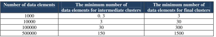
Final clustering threshold defines the percent of the minimum data elements that should be in a final cluster. In the experiments, f-th is a small value, in order to determine the clusters more accurately. Therefore, in the beginning of the data streams, just a few data in a region can make a cluster; gradually over time, the minimum number of data to make a cluster is increased. Table 2 shows the growing rate of the number of data needed to make a cluster (f-th=0. 001).
Table 2) The growing rate of the minimum number of data for clustering
The minimum number of data elements for final clusters The minimum number of
data elements for intermediate clusters Number of data elements
3 0. 3
1000
30 3
10000
300 30
100000
1500 150
500000
As table 2 shows, in the 500000th turn, to cluster a cell it should contain at least 1500 data elements; according to a real experience, in the 80 percent of the real clusters, the number of data elements is less than 1500. So, the f-th for large number of data elements can avoid the determination of small clusters. In order to solve this problem, a periodical adjustment is done on |Dt| as follows:
| D | |D | α α 1 α |D | (14)
αi is num
3. 9. Refi
In our me data set, elements distributi number o data in ea sets, whe order to m
Fig. 5) E
4. Evalua The eval precision the rate o cluster C to Zr. Th solution w Precis Re the FSc In order generated is ranged elements dimensio In order detection The size In the fo experime Windows
Com
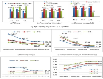
In fig. 6, single pa method f results. T
the number o mber of the gen
finement
ethod, the seq the sequence in each dime ion of a dimen of children an ach dimension en a data set c
minimize the u
Effect of the diffe deviations in
ation luation criteri n and recall. P of correct mat Ci with the ni n
he FScore valu where k is the
sion (correctn
ecall (accuracy
The FScore is
core of the ove
to evaluate th d by the data d over [0,100)
are concent on [Park and L
to show the p n data set [KD
of each dimen llowing, four ents are perfo s Vista and all
mparing "B+
the performan ass algorithms for data stream The conditions
‐ (F-th= ‐ Condi
‐ The D
of the data ele nerated data el
quence of dime e of dimensio ension. They nsion is tightl nd the number
n on the numb contains non-n
unwanted beh
erent sequences o n an ascending or
ia are describ Precision defin tches in the m
number of sim ue of a catego e number of cl
ness) is defined
y) is defined a
s defined as:
erall clustering
he performan generator use ) and the valu trated on ran Lee (2007)].
performance DD Cup (1999 nsion is norma
different exp ormed on a 2 l programs im
C tree" to the
nce of the pro s (online). The ms. The param s of the experi =0. 001, h=10) itions are chec Data set for the
ements that b lements in the
ensions does n ons can be d
can be sorted y concentrate r of nodes are ber of Cluster numerical data haviors in the
f dimensions in th rder. (b) Dimensi
bed as follow nes the rate of model solution. milar data cate ory Zr is the m lusters. A goo
d as:
as:
g solution is:
ce of the prop d in ENCLUS ue of each dat ndomly chose
of proposed m )] is experime alized into [0,
eriments are d 2. 4 GHZ cor mplemented in
e previous alg
oposed algorith e direct comp meters of three iment are as fo ).
cked for refine e experiment i
belong to a fin e constant peri
not have to be determined by
d by the stand ed, the numbe
e reduced. Fig r tree’s nodes. a, the k-means clustering suc
the structure of th ions are sorted by
ws [Zhao and f correct matc . Given a cate egorized. Let maximum FSc od solution has
posed method S [Cheng et a ta element is en 20 data r
method on a r ented. All 41 ,100).
done to evalu re 2 duo Pen n Microsoft Vi
gorithms.
hm is compar parison is don e methods are
ollows:
ement after ea is KDD-CUP’
nal cluster in iod of time.
e preordered. B y monitoring
dard deviation r of the nonad g. 5 shows th . Our algorithm s technique ca ch as breaking
he Clustering tree y the standard dev
d Karypis (20 ches in the ge egory Zr with nri be the num core value atta s the FScore c
d "B+C tree", al. (1999)]. Th randomly sel egions, with
real data set, t continuous at
uate the perfor ntium PC mac isual Studio 20
red with the L e to CS tree w
adjusted to pr
ach 1M data el ’99.
a constant pe
But, based on the standard ns in an ascen djacent cluster e effect of the m is designed an be applied g a cluster into
. (a) Dimensions viations in a desce
002)]: FScore enerated soluti the nr numbe mber of data ained in any c close to one.
,
,
1
∑
, a number of he domain of e ected. In this randomly va
the KDD-CUP ttributes are em
rmance of the chine with 2 005.
SEARCH and which is also
rovide a simil
lements.
eriod of time
our knowledg d deviation of
nding order. ers is decrease
e standard de d for the nume
on the final c o sub-clusters.
are sorted by the ending order.
e is a combi ion, and Reca er of similar d in cluster Ci b cluster of the
,
f synthetic da each dimensio
experiment, aried size in
P’99 network mployed for c
e proposed me GB main m
d CS tree sinc a grid-based lar situation to
over total
ge about a f the data
When the ed. So, the viation of erical data clusters, in e standard ination of all defines data, and a belonging clustering (15) (16) (17) (18)
ata set are onal value most data different k intrusion clustering. ethod. All emory on
The resul usage of slightly m processin average p
Stu
The perf experime The aver accuracy and the m accurate, memory
Stu
Fig. 8 illu the exper
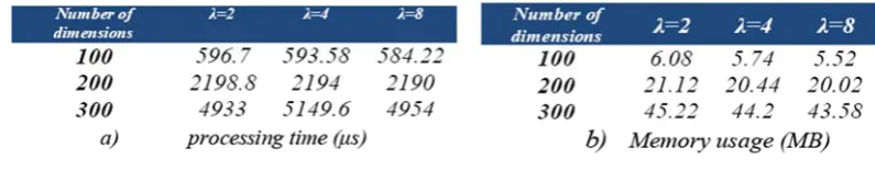
‐ ‐ ‐ ‐ Table 3 dimensio
Stu
Fig. 9 sho are simil which clu other han
lts show an im f our algorithm more than CS ng time is nee processing tim
dying the sca
formance of t ent are the sam rage processin y increases. In
memory usag so the proce used to maint
dying the sca
ustrates the pe riment are as f (F-th=0. 00 Conditions The Data s Number of shows the me on. The algorit
dy the perform
ows the accur ar to the expe usters data wi nd, the accurac
mprovement in m is noticeabl
tree, because eded for clust me per each da
lability of "B
the proposed me as the prev ng time per e n the beginnin ge are increas essing time an tain clusters an
lability of "B
erformance of follows: 01, h=4). s are checked set for the exp f dimensions o emory usage thm has better
mance of "B+
racy of the alg eriment 3. Nu th distinguish cies of other a
n the accuracy ly lower than in our algorit tering. Fig. 6 ata element is
+C tree" on t
method on a ious experime each data elem ng of a data st
sed. With tim nd the memor nd cells is alm
+C tree" on t
f the proposed
for refinemen periment is EN of data stream and the proce r performance
+C tree" on th
gorithm on the umber of clus hed borders, nu
algorithms are
Fig. 6) Compari
y of the cluste the other alg thm, in order t shows, as th decreased.
the number of
a large data s ent. This study ment as well tream, due to me, the algori
ry usage are most not depen
the number of
d algorithm on
nt after each 1 NCLUS. ms is varied fro
essing time ar e on the data w
he number of
e different num sters is varied
umber of clus e decreased be
ing the performan
ering in the pr gorithms. The
to improve th he number of
f data.
stream is show y is done on 4
as the memo the construct thm updates decreased. Fi ndent on the n
f dimensions.
n high dimensi
00M data elem
om 10 to 50. re increased r with less than
f clusters.
mber of cluste d between 4 a
ters is not affe ecause of the i
nce of algorithms
oposed algori processing ti e accuracy an data element
wn in the fig 400,000 data e ry usage decr ion of the tree trees and this g. 7 shows th umber of data
ional data stre
ments.
rapidly by inc 100 dimension
ers. The condi nd 50. For a ected the prop ncrement of c
ithm. Also, the ime of the alg nd memory us
ts is increased
g. 7. Conditio elements.
reases linearl es, the proces s makes clus hat the total a a elements.
eams. The con
creasing the n ons.
itions of the ex data set like posed algorith cluster’s occul
e memory gorithm is age, more d, that the
ons of the
y and the ssing time ters more amount of
nditions of
number of
5. Conclu In this pa of a mu statistics “cluster t arbitrary the proba and size reduced b reduces t
T
usion aper, we propo ulti-dimension
of data elem tree” is propos
shaped cluste ability of clus
of data strea by the define the memory co
Fig. 7
Fig. 8) Compa
Fig. 9) Compar
Table 3) Performa
osed an adapt nal continually ments of data
sed. Our study ers. The clust ster’s overlapp
ams. Also, th ed clustering p
onsumption by
7) the performanc
ring the scalabilit
ring the accuracy
ance of the algorit
tive grid-based y generated d streams, “b+c y over data str er tree mainta ping is almost he number of parameters. F
y increasing th
ce of "B+C tree"
ty of the algorithm
of algorithms on
thm on data strea
d clustering m data stream. cell tree” is de
reams shows t ains the boun t none. The al f data accomm
inally, this al the processing
on the number of
ms on the numbe
n the different num
ams with more tha
method (B+C
In order to efined. To clu that the algori ndaries of mul lgorithm is sc modated for a lgorithm impr g time slightly
f data.
r of dimensions
mber of clusters.
an 100 dimension
tree) to distin maintain the uster high dim ithm is capabl lti dimensiona calable on the appearance of roves the accu
.
ns.
nguish potentia e on-going di
mensional dat le to provide u al clusters pre
number of di f the initial c uracy of clust
References
[1] Agrawal, R.; Gehrke, J.; Gunopulos, D.; Raghavan, P. (1998): Automatic subspace clustering of high dimensional data for data mining applications, in: Proc. of the ACM SIGMOD International Conference on Management of Data, Seattle, Washington, June pp. 94–105. [2] Agrawal, C. C.; Han, J.; Wang, J. (2003): A framework for clustering evolving data streams. In Proc. 29th international conference on
very large data bases, pp. 81–92.
[3] Agrawal, C. C.; Han, J.; Wang, J.; Yu, P. S. (2004): A framework for projected clustering of high dimensional data streams”. In Proc. of 30th international conference on very large data bases, pp. 852–86.
[4] Agrawal, R.; Gehrke, J.; Gunopulos, D.; Raghavan, P. (2005): Automatic Subspace Clustering of High Dimensional Data. Data Mining Knowledge Discovery, Vol. 11, 1, pp. 5-33.
[5] Beringer, J.; Hüllermeier, E. (2003): Online Clustering of Parallel Data Streams, Data & Knowledge Engineering.
[6] Cao F.; Ester M.; Qian W.; Zhou A. (2006): Density-Based Clustering over an Evolving Data Stream with Noise. Proceedings of the SIAM Conference on Data Ming.
[7] Chen Y.; Tu L. (2007): Density-Based Clustering for Real-Time Stream Data. KDD’07, August 12–15, San Jose, California, USA. 133-142.
[8] Cheng, C. H.; Fu, A. W.; Zhang, Y. (1999): Entropy-based subspace clustering for mining numerical data, in: Proc. of ACM SIGKDD International Conference on Knowledge Discovery and Data Mining (KDD-99), San Diego, pp. 84–93.
[9] Guha, S.; Meyerson, A.; Mishra, N.; Motwani, R.; O’Callaghan, L. (2003): Clustering data streams: Theory and practice, IEEE Trans. Knowl. Data Eng. 15 (3), pp. 515–528.
[10] Jae, W. L.; Park, N. H.; Lee, W. S. (2009): Efficiently tracing clusters over high-dimensional on-line data streams, Data & Knowledge Engineering.
[11] Javitz, H. S.; Valdes, A. (1994): The NIDES Statistical Component Description and Justification, Annual Report, A010. [12] Mehta, D. P.; Sahni, S. (2004): Handbook of Data Structures and Applications, Chapman & Hall/CRC, chapter 15.
[13] Muthukrishnan, S. (2003): Data streams: algorithms and applications. Proc. of the fourteenth annual ACM-SIAM symposium on discrete algorithms.
[14] Park, N. H.; Lee, W. S. (2007): Cell trees: an Adaptive Synopsis structure for clustering multi-dimensional on-line data streams, Data & Knowledge Engineering, 63(2), P. P. 528–549.
[15] KDD Cup (1999): <http://kdd.ics.uci.edu/databases/kddcup99/kddcup99.html>.
[16] Thanawin, R.; Komkrit, U.; Kitsana, W. (2007): E-Stream: Evolution-based Technique for Stream Clustering. Springer-verlag Berlin Heidelberg,ADMA, pp. 605-615.