https://doi.org/10.5194/cp-15-1411-2019 © Author(s) 2019. This work is distributed under the Creative Commons Attribution 4.0 License.
Holocene temperature response to external forcing: assessing
the linear response and its spatial and temporal dependence
Lingfeng Wan1,2, Zhengyu Liu3, Jian Liu1,2,4, Weiyi Sun1,2, and Bin Liu1,2
1Key Laboratory for Virtual Geographic Environment, Ministry of Education; State Key Laboratory Cultivation Base of
Geographical Environment Evolution of Jiangsu Province; Jiangsu Center for Collaborative Innovation in Geographical Information Resource Development and Application; School of Geography Science, Nanjing Normal University, Nanjing, 210023, China
2Jiangsu Provincial Key Laboratory for Numerical Simulation of Large Scale Complex Systems, School of Mathematical
Science, Nanjing Normal University, Nanjing, 210023, China
3Atmospheric Science Program, Department of Geography, Ohio State University, Columbus, OH 43210, USA
4Open Studio for the Simulation of Ocean-Climate-Isotope, Qingdao National Laboratory for Marine Science and
Technology, Qingdao, 266237, China
Correspondence:Jian Liu ([email protected]) and Zhengyu Liu ([email protected])
Received: 14 December 2018 – Discussion started: 7 January 2019
Revised: 19 June 2019 – Accepted: 25 June 2019 – Published: 31 July 2019
Abstract.Previous studies show that the evolution of global mean temperature forced by the total forcing is almost the same as the sum of individual orbital, ice sheet, greenhouse gas and meltwater single forcing runs in the last 12 000 years in three independent climate models: Community Climate System Model 3 (CCSM3), Fast Met Office/UK Universities Simulator (FAMOUS) and Loch-Vecode-Ecbilt-Clio-Agism Model (LOVECLIM). This validity of the linear response is useful because it simplifies the interpretation of the climate evolution. However, it has remained unclear if this linear re-sponse is valid on other spatial and temporal scales and, if valid, in what regions. Here, using a set of TraCE-21ka (Sim-ulation of the Transient Climate of the Last 21,000 Years) climate simulations, the spatial and temporal dependence of the linear response of the surface temperature evolution in the Holocene is assessed approximately using the correlation coefficient and a linear error index. The results show that the response of global mean temperature is almost linear on or-bital, millennial and centennial scales in the Holocene but not on a decadal scale. The linear response differs significantly between the Northern Hemisphere (NH) and Southern Hemi-sphere (SH). In the NH, the response is almost linear on a millennial scale, while in the SH the response is almost linear on an orbital scale. Furthermore, at regional scales, the lin-ear responses differ substantially between the orbital,
millen-nial, centennial and decadal timescales. On an orbital scale, the linear response is dominant for most regions, even in a small area of a midsize country like Germany. On a millen-nial scale, the response is still approximately linear in the NH over many regions. Relatively, the linear response is degen-erated somewhat over most regions in the SH. On the centen-nial and decadal timescales, the response is no longer linear in almost all the regions. The regions where the response is linear on the millennial scale are mostly consistent with those on the orbital scale, notably western Eurasian, North Africa, subtropical North Pacific, the tropical Atlantic and the Indian Ocean, likely causing a large signal-to-noise ratio over these regions. This finding will be helpful for improving our under-standing of the regional climate response to various climate forcing factors in the Holocene, especially on orbital and mil-lennial scales.
1 Introduction
or-bital parameters, GHGs, meltwater discharge and continental ice sheet are regarded as external forcing.) Implicit in this in-terpretation is often an assumption that the response is almost linear to the four forcing factors, that is, the temperature evo-lution forced by the total forcing combined is approximately the same as the sum of the temperature responses forced in-dividually by the four forcing factors. This linear response, if valid, simplifies the interpretation of the climate evolution dramatically because each feature of the climate evolution can now be attributed to those on different forcing factors. One example is the global mean temperature evolution of the last 21 000 years (COHMAP members, 1988; Liu et al., 2014). It has been shown that the global mean temperature response is almost linear to the four forcing factors above in three independent climate models (Community Climate System Model 3 (CCSM3), Fast Met Office/UK Universities Simulator (FAMOUS) and Loch-Vecode-Ecbilt-Clio-Agism Model (LOVECLIM); Fig. 2 of Liu et al., 2014) with the temperature evolution forced by the total forcing almost the same as the sum of those individually forced by each forc-ing factor. Furthermore, this deglacial warmforc-ing response is forced predominantly by the increase in GHGs, with sig-nificant contribution from the ice sheet retreat. This linear response, however, has not been assessed quantitatively for the climate evolution in the Holocene. The Holocene period poses a more stringent and interesting test of the linear re-sponse, as it removes the deglacial global warming response that is dominated by that to increased CO2and ice sheet re-treating (Fig. 2a of Liu et al., 2014). An even more interesting and practical question here is, besides the global mean tem-perature response to the slow orbital timescale, how linear is the response at shorter temporal scales and smaller spatial scales, throughout the Holocene?
In general, the assessment of the linear response, in prin-ciple, can be done in a climate model using a set of exper-iments that are forced by the combined forcing as well as each individual forcing. Furthermore, each forcing experi-ment has to consist of a large number of ensemble mem-bers. This follows because a single realization of a coupled ocean–atmosphere model could contain strong internal cli-mate variability on a wide range of timescales (Laepple and Huybers, 2014), from daily variability of synoptic weather storms (Hasselmann, 1976) to interannual variability of El Niño (Cobb et al., 2013) and interdecadal climate variability (Delworth and Mann, 2000), all the way to millennial cli-mate variability (Bond et al., 1997). The ensemble mean is therefore necessary to suppress internal variability and then generate the truly forced response to each forcing. The good-ness of the linear response can therefore be assessed by com-paring the response to the total forcing with the sum of the individual responses. One practical problem with this ensem-ble approach is, however, the extraordinary computing costs, especially for long experiments in more realistic, fully cou-pled general circulation models. A more practical question is therefore: is it possible to obtain a meaningful assessment
of the linear response using only a single realization of each forced experiment for the Holocene, such as those in TraCE-21ka (Simulation of the Transient Climate of the Last 21,000 Years) experiments (Liu et al., 2014).
Strictly speaking, it is impossible to disentangle the forced response from internal variability in a single realization. This would make the assessment of the linear response difficult. However, it is conceivable that, if our interest is the slow climate evolution of millennial or longer timescales in re-sponse to the slow forcing factors such as the orbital forc-ing, ice sheet forcforc-ing, GHGs and meltwater flux, the as-sessment is still possible, albeit approximately, at least for very large-scale variability. This follows because these forc-ing factors are of long timescales and of large spatial scales; the forced response signal should therefore also be on long timescales and large spatial scales if the response is approx-imately linear. An extreme example is the almost linear re-sponse in the global temperature of the last 21 000 years as discussed by Liu et al. (2014). In contrast, internal vari-ability in the coupled ocean–atmosphere system tends to be of shorter timescales (decadal to centennial) and of smaller spatial scales, at least in the current generation of coupled ocean–atmosphere models. This naturally leads to two ques-tions. First, how linear is the climate response at different spatial and temporal scales, quantitatively? Second, in what regions does the linear response tend to dominate? The an-swer to these questions should help improve our understand-ing of regional climate response durunderstand-ing the Holocene. A fur-ther question is as follows: if the linear approximation is valid, what is the contribution of each forcing factor in dif-ferent regions and at difdif-ferent timescales. This question will be addressed in a follow-up paper (Wan et al., 2019).
In this paper, we assess the linear response for the Holocene temperature evolution quantitatively, using five forced climate simulations in CCSM3 (Liu et al., 2014), with the focus on the spatial and temporal dependence of the lin-ear response. We will assess the linlin-earity response to or-bital, millennial, centennial and decadal timescales and on global, hemispheric and regional spatial scales. The data and methodology are given in Sect. 2. The dependence of the linear response to spatial and temporal scales is analyzed in Sect. 3. A summary and further discussions are given in Sect. 4.
2 Data and methods
2.1 Data
Table 1.TraCE-21ka simulation experiments.
No. Experiment Forcing Time Resolution (lat×long.)
1 ORB Orbital forcing 11 000 48×96
2 GHG GHG forcing 11 000 48×96
3 ICE Ice sheets forcing 11 000 48×96
4 MWF Meltwater forcing 11 000 48×96
5 ALL Orbital+GHG+ICE sheet+meltwater forcing 11 000 48×96
GHGs, orbital forcing and meltwater fluxes. The ice sheet is changed approximately once every 500 years, according to the ICE-5G reconstruction (Peltier, 2004). The atmospheric GHG concentration is derived from the reconstruction of Joos and Spahni (2008). The orbital forcing follows that of Berger (1978). The coastlines at the LGM (Last Glacial Max-imum) were also taken from the ICE-5G reconstruction and were modified at 13.1, 12.9, 7.6 and 6.2 ka, after which the transient simulation adopted the present-day coastlines. The meltwater flux follows largely the reconstructed sea level and other paleoclimate information and, in the meantime, recon-ciles the response of Greenland temperature and AMOC (At-lantic Meridional Overturning Circulation) strength in com-parison with reconstructions. More information on the de-tails of the experiment and forcing can be seen in He (2011) or on the TraCE-21ka website http://www.cgd.ucar.edu/ccr/ TraCE/ (last access: 11 July 2019).
The transient simulation under the total climate forcing re-produces many large-scale features of the deglacial climate evolution consistent with the observations (Shakun et al., 2012; Marsicek et al., 2018), suggesting a potentially reason-able climate sensitivity in CCSM3, at global and continental scales. In addition to the all-forcing run (ALL), there are four individual forcing runs forced by the orbital forcing (ORB), the continental ice sheets (ICE), the GHGs (GHG) and melt-water forcing (MWF) (Liu et al., 2014; Table 1). In these four experiments, only one forcing varies the same as in experi-ment ALL, while other forcings/conditions remain the same as at 19 ka. Therefore, this set of experiments can be used to study the linear response of the climate to the four forcing factors. Here, we will only examine the surface temperature response in the Holocene (last 11 000 years).
2.2 Assessment strategy
We will use correlation and normalized root means square er-ror (RMSE) to assess the linear response (see next subsection for details). We note, however, that our assessment of the lin-ear response is approximate. Before introducing the details of the assessment method, it is useful here to make some gen-eral comments on the linear response assessment. As pointed out by one reviewer, strictly speaking, the assessment of the linear response requires one to answer two questions.
Q1 How linear is the response to external forcing?
Q2 What is the relative importance of external forcing vs. internal variability, assuming the response were linear?
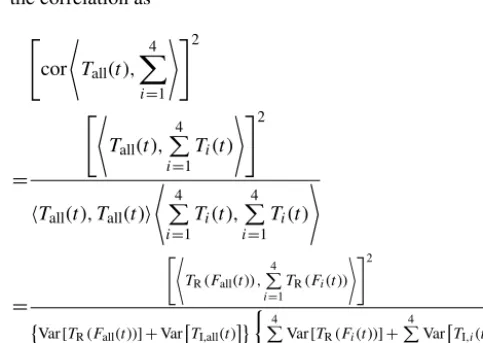
Specifically, for Q1, if we denote the temperature response to the full external forcing byTR(Fall(t)), the response to the individual forcings byTR(Fi(t)) (withi=1, . . .,4), and the internal temperature variability of the five model simulations byTI,all,TI,1,TI,2,TI,3 andTI,4, the linearity of the response could be defined by the extent to which the total forced re-sponse equals the sum of the individual rere-sponses or
TR(Fall(t))= 4
X
i=1
TR(Fi(t)). (1)
In our case, we only have a single member for each experi-ment as
Tall(t)=TR(Fall(t))+TI,all(t)
and
Ti(t)=TR(Fi(t))+TI,i(t),
and the linearity is assessed from the correlation (and nor-malized RMSE) between the sum of the individual
exper-iments 4
P
i=1
Ti(t) and the total forcing experiment Tall(t).
Therefore, our linearity assessment is contaminated by the noise of internal variability. This can be seen, for example, in the correlation as
"
cor *
Tall(t), 4
X
i=1
+#2
=
"*
Tall(t), 4
P
i=1 Ti(t)
+#2
hTall(t), Tall(t)i
*
4
P
i=1 Ti(t),
4
P
i=1 Ti(t)
+
=
"*
TR(Fall(t)), 4
P
i=1
TR(Fi(t))
+#2
Var [TR(Fall(t))]+Var
TI,all(t)
(
4
P
i=1
Var [TR(Fi(t))]+ 4
P
i=1 Var
TI,i(t)
).
Here, h i indicates covariance, and we have assumed that the forced response TR(F∗(t)) and internal variability TI,∗
(where ∗ =all, 1, 2, 3, 4) are independent of each other; in addition, the time series is sufficiently long, so sampling errors are negligible. The correlation therefore depends on the signal-to-noise ratio. If the noise (internal variability) is large, the correlation will be much smaller than 1 even if the response is purely linear as in Eq. (1). The only way to suppress internal variability is to perform a large number of ensemble simulations for each experiment. Given only one member for each experiment, we have to be content that our linear assessment using Eq. (2) is approximate, depending on the signal-to-noise ratio. Related to this problem of sin-gle member experiments, since we cannot distinguish inter-nal variability from forced response clearly, Q2 cannot be assessed exactly either.
In spite of these potential issues, with a single member for each experiment, useful information can still be extracted on linear response. Our general hypothesis is that the slow (or-bital and millennial) and large (continental and basin) vari-ability is composed mostly of forced signal and the faster (centennial and shorter) and smaller variability is mostly as-sociated with internal variability of noise. In other words, in our set of single member of simulations, the signal-to-noise ratio is large for slow variability but small for faster variabil-ity. Qualitatively, this hypothesis seems reasonable. First, all the four external forcing factors are of slow timescales and large spatial scales; additionally, internal variability is usu-ally weak in the coupled ocean–atmosphere system at slow timescales and large spatial scales. Our focus is indeed the slow variability and large scale here, so we can roughly treat the slow and large variability in the single realization as the signal and the linearity of the response may be assessed us-ing Eq. (2). Second, again, because our forcus-ing factors are of slow timescales and large spatial scales, higher-frequency or small-scale variability in the model should not be dominated by the forced variability (unless the response is highly non-linear). Therefore, high-frequency or small-scale variability can be treated roughly as “noise”. This is consistent with the later assessment that slow variability seems to be an approx-imately linear response while high-frequency variability not. Based on this hypothesis, the signal-to-noise ratio is also es-timated using the variance of slow variability as the signal and high-frequency variability as the noise (as in late Fig. 7). It should be noted however that this hypothesis is qualitative in nature. One major purpose of this paper is to give a some-what more quantitative assessment on this hypothesis. How slow, how large and how good will the linear response be?
Our experimental design is proper for linear response as-sessment here. Alternatively, in another experimental setting, individual forcing experiments are often superimposed se-quentially one by one: for example, first the ice sheet, second the ice sheet plus orbital forcing, third the ice sheet, orbital and GHGs, and finally, applying all four forcings of ice sheet, orbital, GHGs and meltwater. In this experimental design, the
full forcing response is by default the response of the sum response after adding the four forcing factors together, and therefore it cannot be used to assess the linearity of the re-sponse. Nevertheless, it should be kept in mind that our four individual forcing experiments are not designed optimally for the study of the linear response in the Holocene. This is be-cause, except for the variable forcing, all the other three forc-ing factors are fixed at the 19 ka condition. As such, the mean state is perturbed from the glacial state, instead of a Holocene state. This may have contributed to some unknown deteriora-tion on the linear response discussed later. Nevertheless, we believe, our major conclusion should hold reasonably well. This is because, partly, the response is indeed almost linear for orbital and millennial variability as will be shown later.
2.3 Methods
We use two indices to evaluate the linear response: the tem-poral correlation coefficientr and a normalized linear error indexLe. The correlation coefficient is calculated as
r=
n
P
t=1
St−St
×Tt−Tt
n s n
P
t=1
St−St
2
n
s n
P
t=1
Tt−Tt
2
n
= cov(St, Tt) σ(St)σ(Tt)
. (3)
Here,St=
4
P
i=1
Ti/4 is the linear sum of the temperature time
seriesTiof the four single forcing experiments,Tt is the full temperature time series in the ALL run (both at timet) and nis the length of the time series. The overbar represents the time mean. The correlation coefficient represents the similar-ity of the temporal evolution between the sum response and the ALL response. However, the correlation does not address the magnitude of the response. Indeed, even ifSt andTt has a perfect correlationr=1, the two time series can still dif-fer by an arbitrary constant in their magnitudes. Therefore, we will also use a normalized linear error indexLeto evalu-ate the magnitude of the linear response. Here,Leis defined as the RMSE of the sum temperature response from the full temperature response divided by the standard deviation of the full temperature response in the ALL run:
Le= RMSE
SD =
s n
P
t=1
[St−St
−Tt−Tt
]2
n s n
P
t=1
[Tt−Tt ]2
n
=σ(St−Tt) σ(Tt)
. (4)
r is sufficiently small andLeis sufficiently large, we cannot confirm the response is either linear or nonlinear because the small ror largeLe can also be contributed by strong inter-nal variability. Second, if the forcing is dominated by shorter timescale variability, say interannual to interdecadal variabil-ity, as in the case of volcanic forcing or solar variabilvariabil-ity, it will be difficult to assess the linear response. This because the timescales of the forced response now overlap heavily with strong internal climate variability in the coupled sys-tem, and it will be difficult to separate the forced response from internal variability without an ensemble mean.
But how to assess the goodness of the linear response from the value ofrandLe? We can test the goodness of the linear response statistically onrandLe.
The statistical significance ofr for a particular timescale is tested using the Monte Carlo method (Kroese, 2011, 2014; Kastner, 2010; Binder, 1997) with 1 000 000 realizations on the corresponding red noise in the AR(1) model (autoregres-sive model of order 1) which uses the AR(1) coefficient de-rived from the model to generate time series. The fit uses the lag-1 auto-correlation coefficient.
The statistical significance of the Le of a particular timescale is tested using a bootstrap method (Efron, 1979, 1993) with 1 000 000 realizations on the corresponding time series. Specifically, the bootstrap is done as follows, taking the global mean temperature as example. First, we will derive theLefrom one random realization on the temperature of the ALL run of the 100 binned data (110 points of data, each representing a 100-year bin). For this random realization, the order of the original temperature time series is swapped ran-domly. Then, this realization is used as a new ALL response for comparison with the sum response of the four individ-ual experiments to derive aLein Eq. (2). Since the random realization distorts the serial correlation time with the sum response, one should usually expect a large error Le. Sec-ond, we repeat this process for 1 000 000 times on 1 000 000 random realizations; this will produce 1 000 000 random val-ues ofLe, forming the PDF of theLe. Third, the minimum 5 % level is then used as the 95 % confidence level.
The dependence of the linear response on spatial and tem-poral scales will be studied by filtering the time series on different scales. For the spatial scale, we will divide the globe into nine successive cases, denoted by nine division factors: f=0, 1, 2, 3, 4, 6, 8, 12 and 24 from the largest global scale to the smallest model grid scale. The f=0 case is for the global average, while the f=1 case is for the hemispheric average in the Northern Hemisphere (NH) and Southern Hemisphere (SH). Further division will be done within each hemisphere. Note that each hemisphere has 96 (long.)×24 (lat) grid boxes, with a ratio of 4 : 1 between longitude span and latitude span. We divide each hemisphere intof×fsections of equal latitude and longitude spans, with each area containing the same number of (96/f)×(24/f) grid boxes, maintaining the ratio of 4 : 1 between longitude span and latitude span. For example,f =2 is for the 2×2
di-vision, with each area containing 48×12 grid boxes;f =24 is for the 24×24 division with each area containing 4×1 grid boxes, about the size of 15◦(long.)×3.75◦(lat), like the
size of a midsize country such as Spain or Germany in the midlatitudes.
On the timescale, we decompose a full 11 000-year annual temperature time series (from 11 to 0 ka) in 100-year bins (a total of 110 data bins or points, each representing a 100-year mean) into three components. The three components are to represent the variability of, roughly, orbital, millennial and centennial timescales. Following Marsicek et al. (2018), we derive the orbital and millennial variability using a low-pass filter called the locally weighted regression fits (Loess fits) (Cleveland, 1979). First, the orbital variability is derived by applying a 6500-year Loess fit low-pass filter to the temper-ature time series, and it therefore contains the trend and the slow evolution longer than∼6500 years. Second, we apply a 2500-year Loess fit low-pass filter onto the temperature time series; then, we derive the millennial variability using this 2500-year low-pass data subtracting the 6500-year low-pass data. Finally, centennial variability is derived as the differ-ence between the 100-year binned temperature time series and the 2500-year low-pass time series. In addition, we also derive a decadal variability time series. First, we compile the 10-year bin time series from the original 11 000-year annual time series (of a total of 1100 data points, each representing a 10-year mean). Second, we apply a 100-year running mean low-pass filter to the time series of the 10-year binned data. Finally, decadal variability is derived by using the 10-year binned time series minus its 100-year running mean time se-ries.
Given the different degrees of freedom especially among the filtered variability of different timescales, it is important to test the goodness of the linear response statistically onr andLe on different timescales differently. As a reference, the significance level is tested against the global mean tem-perature series in the ALL run. For the total, orbital, millen-nial, centennial and decadal temperature time series, the 95 % confidence levels are found to be 0.72 (with the AR(1) coef-ficient 0.96), 0.76 (0.97), 0.65 (0.95), 0.21 (0.31) and 0.19 (0.06), respectively.
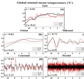
Figure 1.The global annual mean surface temperature time series derived from the ALL run (black) and the SUM (the sum of four single forcing runs, red). In(a), the thin line is the 100-year binned time series; the thick line is 2500-year Loess-fitted time series. The orbital-scale variability(b)is represented by the 6500-year Loess-fitted series. The millennial variability(c)is represented by the 2500-year Loess-fitted data subtracting the 6500-year Loess-fitted data. The centennial variability(d)is represented by the 100-year binned data subtracting the 2500-year Loess-fitted data. The decadal variability (e)is represented by the 10-year binned origin time series subtracting its 100-year running mean. The correlation coefficient (r) is given at the upper left corner and the linear error (Le) is given at the lower left corner of each panel. Thexaxis is year (ka, 0 is 1950 CE), and theyaxis is temperature anomaly (◦C, relative to 11–0 ka).
coefficient is in about the middle of the regional AR(1) co-efficients. The uncertainly of using the global mean AR(1) coefficient is therefore about the average of those of regional AR(1) coefficients. Third, and, most importantly, as our first study here, our focus is on the global features of the linear re-sponse. The difference among the AR(1) coefficients among different spatial scales and different regions is much smaller than that between different timescales here. Therefore, the global mean AR(1) can still provide an approximate guide-line for the proper significant test at different timescales. In later studies, if one’s focus is on a specific spatial scale and on a specific region, the regional AR(1) should be used to reexamine the significance test.
As a reference, the significance level ofLeis tested against the global mean temperature series in the ALL run. For the total, orbital, millennial, centennial and decadal temperature time series, the 95 % confidence levels are found to be 1.23, 1.23, 1.21, 1.24 and 1.36, respectively. This suggests that when the RMSE is less than about 1.2–1.3 times of the
to-tal response, the linear sum is not significantly different from the total response at the 95 % confidence level. As for theLe test, since our focus here is on the global feature of the linear response, for simplicity, the significance level derived from the global mean temperature is used as the common confi-dence level for all regional scales.
3 Results
almost linear on the orbital and millennial scales through-out the Holocene (Fig. 1b and c). The orbital-scale evolu-tion is characterized by a warming trend of about 1◦ from
11 ka to∼4.5 ka before decreasing slightly afterwards. This feature is captured in the linear sum, albeit with a slightly smaller magnitude and an additional local minimum around 3 ka (Fig. 1b). The total variability is very similar to the or-bital variability (r=0.99, Fig. 1a vs. Fig. 1b). The millennial variability shows five major peaks around∼9.8, 7.8, 4.7, 3.7 and 1.8 ka. All these peaks seem to be captured in the sum response, albeit with a slightly larger amplitude (Fig. 1c). For orbital and millennial variability, the correlation coeffi-cients between the sum and the full responses arer=0.83 and 0.71, respectively, both significant at the 95 % confidence level and explaining over 50 % of the variance; the linear er-rors areLe=0.63 and 0.92, respectively, also significant at the 95 % confidence level. It should be noted, however, that the goodness of the linear response is based on the entire period and is meant for the response of the timescale to be studied. Therefore, even for a good linear response at long timescales, the sum response may still differ from the to-tal response significant at some particular time. For exam-ple, for the orbital-scale response in Fig. 1b, even though the linear response is good in terms ofr andLe, there is a 1◦C difference between the sum and total responses at 11 and 3 ka. Therefore, for the orbital-scale response, the linear response mainly refers to the trend-like slow response of the comparable timescale of the orbital scale instead of some re-sponse features of shorter timescales. Further down the scale, at a centennial timescale, the global centennial variability appears also to exhibit a modest linear response (Fig. 1d), withr=0.44 andLe=1.21. But the linear response of the decadal variability becomes poor (Fig. 1e), withr= −0.02 and Le=1.99, which is not statistically significant at the 95 % confidence level. The result of the analysis of global mean temperature is qualitatively consistent with the previ-ous hypothesis that the linear response tends to degenerate at a shorter temporal scale because of the smaller forced re-sponse signal and the presence of strong internal variabil-ity. It shows that, for global temperature, the response is ap-proximately linear at orbital and millennial timescales but be-comes much less so at centennial scales and fails completely at decadal scales.
3.2 Linear responses at different spatial scales
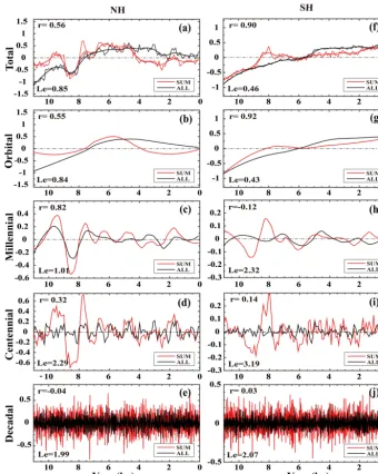
In order to assess the linear response at different spatial scales, we first analyze the linear response to the hemisphere scale for the NH and SH (f =1). It is interesting that the linear response significantly differs between the NH and SH (Fig. 2). Figure 2a and f are the total variability of hemi-spheric surface temperature of the ALL response and sum response for the NH and SH, respectively. Their components on the four timescales (i.e., orbital, millennial, centennial and decadal) are shown in Fig. 2b–e and 2g–j, respectively.
In the NH, the response is almost linear at the millennial scale (r=0.82,Le=1.01, Fig. 2c) but not so strong on or-bital (r=0.55,Le=0.84, Fig. 2b) and centennial (r=0.32, Le=2.29, Fig. 2d) scales, while onlyLeis significant on the orbital scale, and onlyris significant on the centennial scale. At the decadal scale, the linear response fails completely (r= −0.04,Le=1.99, Fig. 2e). In comparison, in the SH, the linear response is dominant at the orbital scale (r=0.92, Le=0.43, Fig. 2g) but poor on all other timescales, in-cluding millennial (r= −0.12,Le=2.32, Fig. 2h), centen-nial (r=0.14, Le=3.19, Fig. 2i) and decadal (r=0.03, Le=2.07, Fig. 2j) scales. The linear response of the global mean temperature discussed in Fig. 1 therefore seems to be dominated by the SH response to the orbital scale but by the NH response to the millennial scale. This suggests that the goodness of the linear response depends on both the region and timescale, highlighting the need to study the linear re-sponse at regional scales.
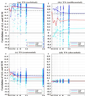
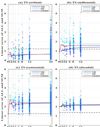
The linear response at different spatial scales and on the orbital, millennial, centennial and decadal timescales is sum-marized in Figs. 3 and 4 in the correlation coefficient and linear error index, respectively. Figure 3a shows the correla-tion coefficients of the orbital variability in each region for the nine division factors. The cases of global mean (f =0) and hemispheric mean (f =1) have been discussed in detail before. The correlation coefficients for succeeding division factors (f =2,3, . . .,24) show several features. First, as ex-pected, the correlation coefficient tends to decrease towards smaller areas (largerf). Quantitatively, however, the corre-lation coefficient does not decrease much, such that even in the smallest area (f =24), the correlation in most regions is still above 0.8, statistically significant at the 95 % con-fidence level. This suggests that the response at the orbital scale is almost linear over most regions, even at the small-est scale of about a midsize country like Germany (f=24, 15◦(long.)×3.75◦(lat)). Second, the linear response in the NH is slightly better than SH (forf ≥3), a topic to be re-turned to later. Third, subareas in both hemispheres show a comparable linear response across all the spatial scales, with the median correlations all above∼0.8, except that of the NH mean temperature (f =1). The linear response of NH is not better than those of regional variability at smaller spatial scales (f ≥2). This is opposite to the expectation that the linear response becomes more distinct for a larger area be-cause the average over a larger area tends to suppress internal variability more. This case, however, seems to be a special feature and should be treated with caution. The correlation coefficient therefore shows that, for orbital-scale evolution, the temperature response is dominated by the linear response over most of the globe, even at regional scales. These features are also consistent with the linear error analysis in Fig. 4a.
re-Figure 2.The surface temperature time series derived from the ALL run (black) and the SUM (red). Panels(a–e)are similar to Fig. 1a–e but for NH, and(f–j)are similar to Fig. 1a–e but for SH. Thexaxis is year (ka, 0 is 1950 CE), and theyaxis is the temperature anomaly (◦C, relative to 11–0 ka).
gions, albeit less so than at the orbital scale. The correlation coefficients remain above 0.6 across most regions even at the smallest division area (f =24), contributing to ∼40 % of the variance. In contrast to orbital variability, where regions in both hemispheres show a comparable linear response, mil-lennial variability shows that the response cannot be con-firmed as linear in most regions in the SH, with the median no longer significant at the 95 % confidence level. Similar to the orbital variability, nevertheless, the responses are more linear in the NH than SH on all the spatial scales.
In contrast to orbital and millennial variability, almost no response can be confirmed as linear for centennial variabil-ity. The median linear response is no longer significant on the centennial timescale in either hemisphere across spatial
scales (f >3, Figs. 3c and 4c), with few correlation coeffi-cients larger than 0.3 and contributing less than 10 % of the variance. Finally, decadal variability exhibits absolutely no linear response over any spatial scales in either the NH or SH (Figs. 3d and 4d).
variabil-Figure 3.Correlation coefficient of mean surface temperature between the ALL and SUM outputs in different spatial timescales.(a)Orbital; (b)millennial;(c)centennial;(d)decadal. The blue dots for NH, cyan dots for SH and red dots for all the correlation coefficient median on the same global spatial scale (i.e., factor). The red line connects the median dots at all division factors. The blue (cyan) line connects the median of all blue (cyan) dots at all division factors. The black thick dashed line is the 95 % confidence level. The black thin solid line is 0. Thexaxis is division factor, and theyaxis is the correlation coefficient. There are only about 10 points with the correlation coefficient lower than−0.5 so they are ignored in(a–c).
ity may also be contributed by nonlinear responses of the climate system. But, given the almost complete absence of forcing variability at this short timescale in our experiments, we do not think that the nonlinear response is the major cause of the poor linear response here.
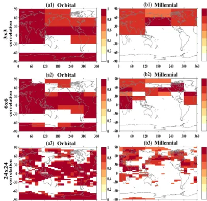
3.3 Pattern of the linear responses
We now further study the pattern of the linear response. Fig-ure 5 shows the spatial patterns of the correlation coefficients at orbital (Fig. 5a1–a3) and millennial (Fig. 5b1–b3) scales for three representative spatial scales: f =3, 6 and 24 (the other factors are not shown because they are similar to the abovementioned three representative spatial scales). For or-bital variability (Fig. 5a1–a3), the response is almost
Figure 4.Same as Fig. 3 but for linear error (Le,yaxis). The black thick dashed line is 95 % confidence level ofLe. There are only about 10 points with theLelarger than 6, so they are ignored in(a–c).
North Africa, Central and South America, most NH oceans and SH tropical oceans, and the Antarctic continent, as seen in Fig. 5a2 and a3 (only significant correlation coefficients are shown). But the linear response is poor over the North America continent and the eastern Eurasian continent, and the entire Southern Ocean. Similar features can also be seen in the map of linear error (not shown).
For millennial variability, in the NH, the linear response shows a similar feature to that of orbital variability, but the linear response is poor over almost all the SH. Figure 5b1–b3 show that the response is almost linear in most regions in the NH at the three spatial scales, with the correlation coefficient above 0.6. At the regional scale, e.g.,f =6 and 24 (Fig. 5b2 and b3), the response is almost linear over the
Figure 5.Correlation coefficient of mean surface temperature between the ALL and SUM outputs of the two timescales (a1–a3, orbital; b1–b3, millennial) for three representative spatial scales:f=3, 6 and 24 (the other factors are not shown because they are similar to the abovementioned three representative spatial scales). Only those regions significant at the 95 % confidence level are shaded in colors.
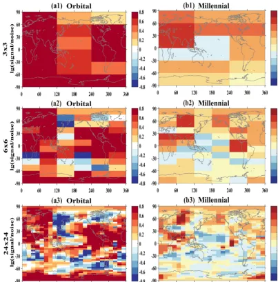
linear response potentially suggests some common mecha-nisms of the climate response in these regions, in this model. In order to understand the cause of the preferred regions of the linear response, we examine the signal-to-noise ratio. As discussed in Sect. 2.2, our forcing factors are on millennial and orbital timescales, and the linear response is also largely valid for orbital and millennial variability. We will therefore use the variance of the orbital and millennial variability as a crude estimate of the linear response signal. Similarly, since there is no centennial and decadal forcing in our model and the response of centennial and decadal variability is not a lin-ear response, we use the variance of the sum of the centen-nial and decadal variability as a rough estimate for internal variability as the linear noise. Admittedly, this estimation is crude, limited by the single realization here. This signal-to-noise ratio does not directly address Q2 in Sect. 2.2 because the timescales of the signal and noise are different. Instead,
Figure 6.The signal-to-noise ratios on the orbital(a1–a3)and millennial(b1–b3)timescales derived from the ALL run. Here the signal is used by the orbital (millennial) variability variance, and the noise is used by the sum of the centennial and decadal variabilities variance. The numbers of 1, 2 and 3 are for the three representative spatial scales:f=3, 6 and 24, respectively. In order to show the signal clearly, the log base 10 is taken on the signal-to-noise ratios.
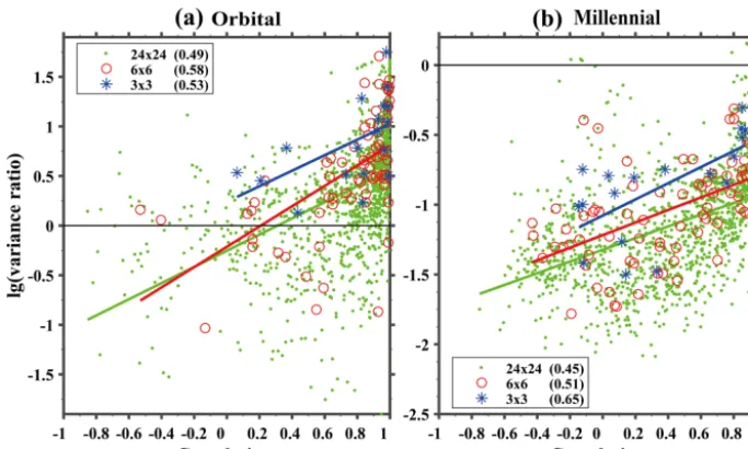
ratio is small over Canada and the eastern Eurasian conti-nent, and the entire Southern Ocean. These spatial features of signal-to-noise ratio on the orbital scale (Fig. 6a1–a3) are similar to those in the correlation map (Fig. 5a1–a3). The spatial correlation between the map of the signal-to-noise ra-tio in Fig. 6 and the corresponding correlara-tion coefficient in Fig. 5 is 0.53, 0.58 and 0.49 forf =3, 6 and 24, respectively, as seen in the scatter diagram in Fig. 7, all significant at the 95 % confidence level.
For millennial variability, the signal-to-noise ratio also shows a similar feature to that of orbital variability although overall somewhat smaller (note the different color scales). Figure 6b1–b3 show that the signal-to-noise ratio is large in most regions in the NH in all three spatial scales, with the
Figure 7.Scatter diagram of the correlation coefficient and the signal-to-noise ratio (variance ratio) on the orbital(a)and millennial(b) timescale. The log base 10 is taken on the variance ratio, as indicated in Fig. 6. Only the three representative spatial factors (f=3, 6 and 24) are shown in the panels. The blue stars and linear fitting line are for factor 3; the red circles and linear fitting line are for factor 6; the green dots and linear fitting line are for factor 24. The fitting coefficients are listed in the brackets at the upper left corners of(a)in the lower left corner of(b).
North Pacific, the North Atlantic and the tropical north Indian Ocean. These features of the spatial pattern of signal-to-noise ratio on the millennial scale (Fig. 6b1–b3) are similar to those in the correlation map (Fig. 5b1–b3). The correlation coeffi-cient between the maps of signal-to-noise ratio and correla-tion is 0.65, 0.51 and 0.45 forf =3, 6 and 24, respectively (Fig. 7), again all significant at the 95 % confidence level.
4 Summary and discussions
In this paper, the linear response is assessed for the surface temperature response to orbital forcing, GHGs, meltwater discharge and continental ice sheet throughout the Holocene in a coupled GCM (general circulation model; CCSM3). The global mean temperature response is almost linear on the or-bital, millennial and even centennial scales throughout the Holocene but not for decadal variability (Fig. 1). Further-more, the sum response accounts for over 50 % of the to-tal response variance for orbito-tal and millennial variability. Further analysis on the regional scale suggests that the re-sponse is approximately linear on the orbital and millennial scales for most continental regions over the NH and SH, with the sum response explaining over about 50 % of the total re-sponse variance. However, the linear rere-sponse is not signif-icant over much of the ocean, especially over the ocean in the SH. There are specific regions where the linear response tends to be dominant, notably the western Eurasian conti-nent, North Africa, central and South America, the Antarctic continent, and the North Pacific. The strong linear response is interpreted as the region of large signal-to-noise ratio. That
is, in these regions, either the orbital and millennial response signal is large or the influence of the centennial and decadal variability noise is small or both. This suggests that the or-bital and millennial variability in these regions is relatively easy to understand. This finding lays a foundation for our fur-ther understanding of the impacts of different climate forc-ing factors on the temperature evolution in the Holocene of orbital and millennial timescales. This understanding is our original motivation for this work. Further work is underway in understanding the contribution of different forcing factors on the temperature evolution (Wan et al., 2019).
assess-ment of the linear response for the Holocene and can serve as a starting point for further studies in the future.
There are many further issues that need to be studied. Our study here is carried out for a single variable (surface tem-perature) in a single model (CCSM3) for the Holocene. Yet, the linear response could differ for different variables, in dif-ferent models, for difdif-ferent periods and for difdif-ferent sets of forcing factors. For example, if we evaluate the precipitation response in the Holocene in CCSM3, the response is less lin-ear than temperature (not shown); this is expected because the precipitation response contains more internal variability and exhibits more nonlinear behavior than temperature. The assessment will be also different if a different period is as-sessed, e.g., the last 21 000 years; with a large amplitude of climate forcing, the linear response may degenerate in the 21 000-year period. In addition, the assessment of the linear response using only one realization will be difficult to per-form for volcanic forcing and solar variability forcing; these forcing factors have short timescales and therefore their im-pacts will be difficult to separate from internal variability without ensemble experiments. Finally, it is also important to repeat the same assessment here in different models and to establish the robustness of the assessment. It should also be kept in mind that our assessment is implicitly related to the assumption that, at millennial and orbital timescales, inter-nal variability is not strong relative to the forced responses. Although this seems to be consistent in our model, there is a possibility that internal variability is severely underestimated in the model compared to the real world (Laepple and Huy-bers, 2014). If true, the relevance of our model assessment to the real world will be limited. It should also be kept in mind that, if the response is dominated by that to a single forcing, the assessment of the linear response here becomes one that is more relevant to the question of the forced response vs. in-ternal variability, as discussed in Q2 in Sect. 2.2. As a further step, though, one can examine if the magnitude of the total response responds to the magnitude of this single forcing lin-early.
Even in the context of this model assessment, much fur-ther work remains. Most importantly, the purpose of testing the linear response is for a better understanding of the physi-cal mechanism of the climate response. It is highly desirable to understand why the response tends to be linear in some re-gions but not in others. In particular, it is unclear why the linear response is preferred over land than over ocean for orbital and millennial variability. At such a long timescale, one would expect that the upper-ocean response has reached quasi-equilibrium and therefore the surface temperature re-sponse over land and over ocean should not be too different. Ultimately, we would like to assess and understand the phys-ical mechanism of the climate evolution in different regions. This work is underway (Wan et al., 2019).
Data availability. The TraCE-21ka data sets were provided by NCAR from their website at https://www.earthsystemgrid.org/ project/trace.html (last access: 11 July 2019).
Author contributions. LW, JL and ZL conceived the idea for the paper; LW carried out the analysis and prepared the first draft. ZL contributed great ideas and gave the suggestion for the analysis. JL and ZL revised the paper several times. WS provided some useful suggestions to the paper. BL helped to download the larger TraCE-21ka data. All coauthors helped to improve the paper.
Competing interests. The authors declare that they have no con-flict of interest.
Acknowledgements. The authors thank Kai Ding for checking the grammar of the first draft. The TraCE-21ka data sets were pro-vided by NCAR.
Financial support. This work was jointly supported by the Na-tional Key Research and Development Program of China (grant no. 2016YFA0600401), the National Natural Science Foundation of China (grant no. 41420104002, 41630527), the Program of Inno-vative Research Team of Jiangsu Higher Education Institutions of China and the Priority Academic Program Development of Jiangsu Higher Education Institutions (grant no. 164320H116), and NSF OCN1810681.
Review statement. This paper was edited by Qiuzhen Yin and reviewed by Oliver Bothe and two anonymous referees.
References
Berger, A.: Long-term variations of daily insola-tion and quaternary climate changes, J. Atmos. Sci., 35, 2362–2367, https://doi.org/10.1175/1520-0469(1978)035<2362:LTVODI>2.0.CO;2, 1978.
Binder, K.: Applications of Monte Carlo methods to statistical physics, Rep. Progr. Phys., 60, 487–559, https://doi.org/10.1088/0034-4885/60/5/001, 1997.
Bond, G., Showers, W., Cheseby, M., Lotti, R., Almasi, P., de Menocal, P., Priore, P., Cullen, H., Hajdas, I., and Bo-nani, G.: A Pervasive Millennial-Scale Cycle in North At-lantic Holocene and Glacial Climates, Science, 278, 1257–1266, https://doi.org/10.1126/science.278.5341.1257, 1997.
Cleveland, W. S.: Robust Locally Weighted Regression and Smoothing Scatterplots, Journal of the American Statistical As-sociation, 74, 829–826, https://doi.org/10.2307/2286407, 1979. Cobb, K. M., Westphal, N., Sayani, H. R., Watson, J. T., Lorenzo,
COHMAP Members: Climatic Changes in the Last 18,000 Years: Observations and Model Simulations, Science, 241, 1043–1052, https://doi.org/10.1126/science.241.4869.1043, 1988.
Delworth, T. L. and Mann, M. E.: Observed and simulated multi-decadal variability in the Northern Hemisphere, Clim. Dynam., 16, 661–676, https://doi.org/10.1007/s003820000075, 2000. Efron, B.: Bootstrap Methods: Another Look at the Jackknife, Ann.
Stat., 7, 1–26, https://doi.org/10.1214/aos/1176344552, 1979. Efron, B. and Tibshirani, R. J. (Eds.): An introduction to the
boot-strap, Chapman and Hall/CRC, New York, 1993.
Hasselmann, K.: Stochastic climate models Part I, Theory, Tellus, 28, 473–485, https://doi.org/10.3402/tellusa.v28i6.11316, 1976. He, F.: Simulating Transient Climate Evolution of the Last Deglaciation with CCSM3, PhD thesis, Univ. Wisconsin- Madi-son, 1–177, 2011.
Joos, F. and Spahni, R.: Rates of change in natural and anthropogenic radiative forcing over the past 20,000 yearsm P. Natl. Acad. Sci. USA, 105, 1425–1430, https://doi.org/10.1073/pnas.0707386105, 2008.
Kastner, M.: Monte Carlo methods in statistical physics: mathe-matical foundations and strategies, Commun. Nonlinear Sci., 15, 1589–1602, https://doi.org/10.1016/j.cnsns.2009.06.011, 2010. Kroese, D. P., Brereton, T., Taimre, T., and Botev, Z. I.: Why the
Monte Carlo method is so important today, WIRES Comput. Stat., 6, 386–392, https://doi.org/10.1002/wics.1314, 2014. Kroese, D. P., Taimre, T., and Botev, Z. I. (Eds.):
Hand-book of Monte Carlo Methods, Wiley Series in Proba-bility and Statistics, John Wiley and Sons, New York, https://doi.org/10.1002/9781118014967, 2011.
Laepple, T. and Huybers, P.: Ocean surface temperature vari-ability: Large model-data differences at decadal and longer periods, P. Natl. Acad. Sci. USA, 111, 16682–16687, https://doi.org/10.1073/pnas.1412077111, 2014.
Liu, Z., Otto-Bliesner, B. L., He, F., Brady, E. C., Tomas, R., Clark, P. U., Carlson, A. E., Lynch-Stieglitz, J., Curry, W., Brook, E., Erickson, D., Jacob, R., Kutzbach, J., and Cheng, J.: Transient Simulation of Last Deglaciation with a New Mech-anism for Bølling-Allerød Warming, Science, 325, 310–314, https://doi.org/10.1126/science.1171041, 2009.
Liu, Z., Zhu, J., Rosenthal, Y., Zhang, X., Otto-Bliesner, B. L., Timmermann, A., Smith, R. S., Lohmann, G., Zheng, W., and Elison, T. O.: The Holocene tempera-ture conundrum, P. Natl. Acad. Sci. USA, 111, 3501–3505, https://doi.org/10.1073/pnas.1407229111, 2014.
Marsicek, J., Shuman, B. N., Bartlein, P. J., Shafer, S. L., and Brewer, S.: Reconciling divergent trends and millen-nial variations in Holocene temperatures, Nature, 554, 92–96, https://doi.org/10.1038/nature25464, 2018.
Peltier, W. R.: Global Glacial Isostasy and the Sur-face of the Ice-Age Earth: The ICE-5G (VM2) Model and GRACE, Annu. Rev. Earth Pl. Sc., 20, 111–149, https://doi.org/10.1146/annurev.earth.32.082503.144359, 2004. Shakun, J. D., Clark, P. U., He, F., Marcott, S. A., Mix, A.
C., Liu, Z., Otto-Bliesner, B., Schmittner, A., and Bard, E.: Global warming preceded by increasing carbon dioxide con-centrations during the last deglaciation, Nature, 484, 49–54, https://doi.org/10.1038/nature10915, 2012.