ENHANCING THE COMPUTATIONAL
PERFORMANCE OF
NEWTON-RAPHSON POWER FLOW CODES IN
POWER SYSTEM PROBLEMS
A.PRASAD RAJU
Assoc. Professor in EEE Dept., Sree Chaitanya Institute of Technological Sciences, LMD Colony,Karimnagar,A.P , 505527,India.
PROF. J. AMARNATH
EEE Dept., J N T U H College of Engineering, Hyderabad, A P, 500085, India. [email protected]
PROF.D. SUBBARAYUDU
EEE Dept., G.Pulla Reddy Engineering College, Kurnool-02, A.P, India
Abstract :
Power flow studies of power systems give the important computations procedures to find the present operational characteristics and loading predictions which are useful for future planning of the system according to the growing demand. Newton Raphson method is a very popular one to compute the solution of power flow problem due to its fast convergence in few iterations. Jacobins of the Newton Raphson method to be solved in a simple, faxable and reliable manner to evaluate the accurate values. This paper describes a powerful technique known as Automatic Differentiation (AD), applied to compute first order partial derivatives or Jacobin elements that occur in Newton Raphson method when solving power flow problem. Evaluation of the derivatives obtained for the expressions specified in the form of computer program, in a way such that code is differentiated rather than expression, unlike in the traditional finite differentiation. Main program of Newton Raphson power flow method is exempted from the tedious task of computing error full Jacobian partial derivatives and makes the calls to a well defined AD tool to do this task accurately whenever required. This loose coupling between main program and AD code enhances the computational performance and create a flexible solution environment to compute the load flow solutions efficiently. In this paper Automatic Differentiation technique is explained in context to power flow, and then demonstrated on a 4-bus test system and simulation results have been compared and analyzed.
Keywords: Newton Raphson power flow, Jacobians, Automatic Differentiation (AD), AD Too, ADMAT.
1. Introduction
2. Formation of Power flow Model
To apply the popular Newton Raphson method to solve the Power flow equations, consider a power system network with a finite number of buses. Let say that power transfer is occurring between kth bus and mth bus as shown in Fig.1. The power mismatch at the kth bus given as:
Fig.1 Representation of small portion of power system network
0
= − −
=PGK PLK Pkcal k
ΔP (1)
0
=
−
−
=
Δ
Q
kQ
GKQ
LKQ
kcal (2)Where
Δ
Pk,Δ
Qk describes the active and reactive power mismatch, PGk, QGk are the active, reactive power generation and PLk, QLk refer’s the active, reactive power loads, specified at kth bus respectively. Finally Pkcal, Qkcal are the unspecified active, reactive powers transmitted, between kth and mth bus known as power flow equations given with respect to nodal voltages (Vk, Vm) phase angles (θ
k,θ
m), and line impedances, as shown:(
)
(
)
[
km k m km k m]
m k kk k
kcal
V
G
V
V
G
B
P
=
2+
cos
θ
−
θ
+
sin
θ
−
θ
(3)(
)
(
)
[
km k m km k m]
m k kk k
kcal
V
B
V
V
G
B
Q
=
−
2+
sin
θ
−
θ
−
cos
θ
−
θ
(4)Where k=m= 1,2,………nb, as nb is number of buses and bus1 is slack bus. Applying Newton – Raphson method to the solution of power flow problem, power mismatch equation’s or power balance equations of eq (1) & (2) are written as shown below.
Δ
Δ
∂
∂
∂
∂
∂
∂
∂
∂
=
Δ
Δ
V
V
V
V
Q
Q
V
V
P
P
Q
P
θ
θ
θ
(5)F
(
X
(i-1))
J
(
X
(i-1))
∆
X
(i)It is clear from eq (5) that the terms representing the J(X(i-1)) are the Jacobian elements which are the Partial derivatives of real and reactive powers with respect to the known state variables X (V and θ). Proper selection of initial values for X is important factor to reduce iterative process, which will be continued until ∆X given in eq. (6) attains the value that should be within the prescribed tolerance. And at this popint X(i) (V’s, ∆’s) given in eq. (7) gives the feasible solution of load flow problem.
( )
(
1))
( )
( )1 1)
(
=
−
− − −Δ
i i iX
F
X
J
X
Q
(6)
( )i X( )i AX( )i
X = −1 + (7)
3. Automatic Differentiation:
As the conventional differentiating approaches have the many draw backs like occurrence of approximated values with truncation errors, high computational expenses in calculating derivatives leads towards unfair solutions.In further stages the interplay between derivatives computation, large scale non liner power system application and numerical optimization, develops an inefficient, variety final solution. Automatic Differentiation (AD) on the other hand facilitates effective way of accurate evaluation of derivatives of functions, represented in the form of program using high level programming languages[7]. Some of the advantages of AD over other differentiation techniques are (i) It computes the derivatives of the code which represents the function, rather than function directly, by combining the derivatives of elementary operations whose derivatives are already known. It reduces the complexity and memory allocation which leads towards reduction in cost of computation and work load of computation. (ii) AD computes the exact values of derivatives very accurately up to machine precision and relived from the nuisance of having, approximated values of derivatives with truncation errors. (iii)The main program of power flow is relieved from the burden of computing complex derivatives and assigned it to powerful AD tool, the loose coupling between these two codes increases the flexibility and efficiency of the computing environment. (iv) Parallel computing of derivatives is possible using multithreading concepts of High level programming languages, instead of serial computing, which further reduces the processing time as well as cost of the computation increasing the performance of the derivative computation. Powerful AD Tools were developed in different high level programming languages like Fortran, C, C++, MATLAB, Java to evaluate First Order, Second Order derivative efficiently. Some of the popular AD tools are ADIFOR, ADOL, ADMAT and ADiJaC etc.
3.1 Technique of Automatic Differentiation:
In Automatic Differentiation every function is expressed as computer program by decomposing it as a long sequence of simple elementary operations (such as multiplication, Addition and subtraction) and intrinsic functions (like sin, cos, exp etc.) in the form of statements, whose derivatives are already known. Chain rule of differentiation allows these stepwise derivatives to be combined to give the whole derivative of a given function which is coded as a program using high level languages such as C, C++, MATLAB and Java[8-9]. The chain rule which allows decomposition of differentials is givens as:
( )
∂
∂
∂
∂
=
∂
∂
= =
=0 0 0
)
(
)
(
)
(
)
(t t t
g s t
t
t
t
g
s
s
f
t
t
g
f
(8)
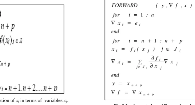
Let consider a function y=f(x), where f:Rn R, then the subroutine shown in Fig. 2, explains that the function f(x) is a composition of elementary functions
{ }
P n
n i i
f
=++1such that fi is function with already computed quantities xj, j€Ji, where xj’s are known as the intermediate variables.
Fig. 2 Representation of xi in terms of variables xj.
Fig.3 Implementation of Forward mode AD
Two well known strategies of Automatic Differentiation are (i) Forward mode (ii) Revenge mode. Here in this paper the scope is restricted to demonstrate the forward mode Automatic Differentiation only. In the forward mode approach , gradient object ∆xi is associated with each scalar variable xi in the code, such that ∆xi always accommodate the derivatives of xi with respect to the intermediate variables xj, as shown in the below given code snippet of Fig.3.
p n p n
j J
j j
i i
i j
i i
i i
x f
x y end
x x
f x
J j ) x ( f x
p n : n i for end
e x
n : i for
) x , f , y ( FORWARD
i
+ +
∈
∇ = ∇
=
∇
∂ ∂ =
∇
∈ =
+ +
= = ∇
=
∇
4. Application of AD Technique to Power Flow Function
Consider a small part of Power System Network contains two buses k and m as shown in Fig1. Then the active Power transfer Pkcal is gives as equation 3. This can be rewritten as
(
)
(
)
[
km k m km k m]
m k kk k
kcal
V
G
V
V
G
B
P
=
2+
cos
θ
−
θ
+
sin
θ
−
θ
(9)
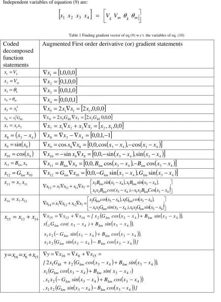
Independent variables of equation (9) are:
[
]
=
V
kV
m k mx
x
x
x
1 2 3 4θ
θ
(10)
Table 1 Finding gradient vector of eq (9) w.r t. the variables of eq. (10)
Coded
decomposed
function
statements
Augmented First order derivative (or) gradient statements
k
V
x1=
∇
x
1=
[
1
,
0
,
0
,
0
]
m
V
x2=
∇
x
2=
[
0
,
1
,
0
,
0
]
k
x3=θ
[
0
,
0
,
1
,
0
]
3=
∇
x
m
x4=θ
∇
x
4=
[
0
,
0
,
0
,
1
]
21 5 x
x =
∇
x
5=
2
x
1∇
x
1=
[
2
x
1,
0
,
0
,
0
]
kkG x
x6= 12 ∇x6 =2x1Gkk∇x1=
[
2x1Gkk0,0,0]
2 1 7 xx
x =
[
,
,
0
,
0
]
1 2 1 2 2 1
7
x
x
x
x
x
x
x
=
∇
+
∇
=
∇
(
3 4)
8
x
x
x
=
−
∇
x
8=
∇
x
3−
∇
x
4=
[
0
,
0
,
1
,
−
1
]
( )
8 9sin
x
x
=
∇
x
9=
cos
x
8∇
x
8=
[
0
,
0
,
cos
(
x
3−
x
4)
,
−
cos
(
x
3−
x
4)
]
( )
910
cos
x
x
=
∇
x
10=
−
sin
x
8∇
x
8=
[
0
,
0
,
−
sin
(
x
3−
x
4) (
,
sin
x
3−
x
4)
]
9 11 B x
x = km
∇
x
11=
B
km∇
x
9=
[
0
,
0
,
B
kmcos
(
x
3−
x
4)
,
−
B
kmcos
(
x
3−
x
4)
]
1012
G
x
x
=
km∇
x
12=
G
km∇
x
10=
[
0
,
0
,
−
G
kmsin
(
x
3−
x
4)
,
G
kmsin
(
x
3−
x
4)
]
11 7 13
x
x
x
=
(
)
(
)
(
)
− − − − − = ∇ + ∇ = ∇ 4 3 2 1 4 3 2 1 4 3 1 4 3 2 7 11 11 7 13 x x Cos B x x ), x x cos( B x x , x x sin B x , x x sin B x x x x x x km km km km 12 7 14 x xx =
(
)
(
)
(
)
− − − − − = ∇ + ∇ = ∇ 4 3 2 1 4 3 2 1 4 3 1 4 3 2 7 12 12 7 14 x x sin G x x ), x x sin( G x x , x x cos G x , x x cos G x x x x x x km km km km 14 13 15x
x
x
=
+
(
(
)
(
)
)
(
)
(
G cos(x x ) B sin x x)
, x , x x sin B x x cos G x [ x x x km km km km 4 3 4 3 1 4 3 4 3 2 14 13 15 − + − − + − = ∇ + ∇ = ∇ 15 6 16x
x
x
y
=
=
+
(
)
(
)
(
)
(
)
(
)
(
)
(
)
(
3 4 3 4)
2 1 4 3 4 3 1 4 3 4 3 2 1 15 6 16 2 x x cos B x x sin G x x , x x sin( B x x cos G x , x x sin B x x cos G x G x [ x x x y km km ) km km km km kk − + − − − + − − + − + = ∇ + ∇ = ∇ = ∇
(
)
(
)
(
G sinx x B cosx x)
] xx
, 1 2 km 3− 4 − km 3− 4
(
)
(
)
(
)
(
)
(
)
Substituting in eq (10) gives:
(
)
(
)
[
3 4 3 4]
2 1 2
1
G
x
x
G
cos
x
x
B
sin
x
x
x
P
y
=
kcal=
kk+
km−
+
km−
(11)The gradient vector is given as:
∂
∂
∂
∂
∂
∂
∂
∂
=
∇
=
∇
4 3 2 1x
y
x
y
x
y
x
y
P
y
kcal (12)Using basic elementary arithmetic rules and elementary function, eq. (12) can be decomposed in to simple and small elementary functions as shown in first column of Tables 1, its derivative or gradient also computed as shown in the second column of table 1 such that, accurate values of the function and derivatives were provided simultaneously, instantly and systematically as given in the Table 1.
From table 1 it is observed that final derivative vector or gradient vector of output y,
∇
y is given as(
)
(
)
(
G
cos
x
x
B
sin
x
x
)
,
x
(
G
cos
(
x
x
)
B
sin
(
x
x
)
)
,
x
G
x
[
y
=
2
1 kk+
2 kim 3−
4+
km 3−
4 1 km 3−
4+
km 3−
4∇
(
)
(
)
(
G
sin
x
x
B
cos
x
x
)
,
x
x
(
G
sin
(
x
x
)
B
cos
(
x
x
)
)
]
x
x
1 2−
km 3−
4+
km 3−
4 1 2 km 3−
4−
km 3−
4 (14)Substituting eq (10) in eq (14) we get
(
)
(
)
(
G
cos
B
sin
)
,
V
(
G
cos
(
)
B
sin
(
)
)
,
V
G
V
[
P
y
=
∇
kcal=
k kk+
m kimθ
k−
θ
m+
kmθ
k−
θ
m k kmθ
k−
θ
m+
kmθ
k−
θ
m∇
2
(
)
(
)
(
G
sin
B
cos
)
,
V
V
(
G
sin
(
)
B
cos
(
)
)
]
V
V
k m−
kmθ
k−
θ
m+
kmθ
k−
θ
m k m kmθ
k−
θ
m−
kmθ
k−
θ
m (15) In the case of differentiation of multiple functions of a system of y=f(x) where f: RnRm then ∇ ∇ ∇ ∂ ∂ ∂ ∂ ∂ ∂ ∂ ∂ ∂ ∂ ∂ ∂ ∂ ∂ ∂ ∂ ∂ ∂ = ∇ ∇ ∇ n n m m m n n m x x x x y x y x y x y x y x y x y x y x y y y y . . . . ... . . ... ... . . . 2 1 2 1 2 2 2 1 2 1 2 1 1 1 2 1 (16)
In this context, for a ‘m’ node power system with ‘n’ variables like nodal voltages (v’s) and angles (θ’s), and with the real power flow’s P1, P2, ... Pm ,assuming node 1 as slack bus, the real power derivatives are
∇ ∇ ∇ ∇ ∂ ∂ ∂ ∂ ∂ ∂ ∂ ∂ ∂ ∂ ∂ ∂ ∂ ∂ ∂ ∂ = ∇ ∇ n n . . n m m m m m n n m . . . v v P ... P V P ... V P . . . P .... P V P ... V P P . . . . P θ θ θ θ θ θ 2 2 2 2 2 2 2 2 2 2 1 (17)
Similarly for reactive power gradients also we can develop equations as using the concepts discussed above. And the final derivative vector is similar to the eq.(17), is given below by eq.(18).
∇ ∇ ∇ ∇
∂ ∂ ∂
∂ ∂ ∂ ∂
∂
∂ ∂ ∂ ∂ ∂ ∂ ∂
∂
=
∇ ∇
n n . .
n m m
m m m
n n
m .
. . v v
Q ... Q V Q ... V Q . . .
Q .... Q V Q ... V Q
Q . . . .
Q
θ θ
θ θ
θ θ
2 2
2 2
2
2 2 2
2 2 1
(18)
Eq (18) represents the Jacobean of Nodal powers Q2, Q3 …. Qm which can be solved by the Automatic Differentiation technique as explained above very simply accurately, instantly simultaneously and systematically.
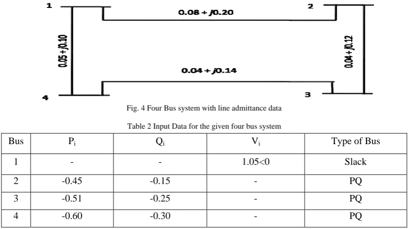
6. Demonstration of AD Technique on a Test System
Automatic Differentiation technique is applied to a 4 bus test system to demonstrate its effectiveness in computing first order derivatives i.e. Jacobian elements occurs in Power flow solution to solve nodal voltages, angles, real and reactive power at each bus using Newton Raphason method. The test system is as shown in the Fig.4 and input data for the given 4 bus system is given in table 2. To find the feasible solution of Power flow problem, Newton – Raphason approach given by equation (19) for 4 bus system to be solved assuming appropriate initial values for independent variables like voltages (v’s) and load angles (θ’s), assuming bus 1 as the slack bus. It is clear from eq.(19) that, the Jacobian matrix containing the derivative elements, should be solved for every iteration until the convergence, to achieve the final solution of Power flow problem.
Fig. 4 Four Bus system with line admittance data
Table 2 Input Data for the given four bus system
Automatic Differentiation in Forward mode approach is applied to solve Jacobian elements, using the popular AD tool ADMAT, written in MATLAB programming language. Main program of Newton Raphason Power flow solution also developed in MATLAB programming environment such that it is relieved from the tedious computational work load of calculating derivative elements and concentrate only on the computation of power mismatch values, Ybus formation, controlling generator limits and matrix operations etc. Computation of Jacobian elements is attended by AD tool ADMAT, upon getting call from main program, whenever, at any point it is required. And well developed functions of ADMAT will complete this assigned task simply, efficiently and returns the accurate, error less values of derivatives to the main program for further usage.
Bus Pi Qi Vi Type of Bus
1 - - 1.05<0 Slack
2 -0.45 -0.15 - PQ
3 -0.51 -0.25 - PQ
2
P
Δ
=
2 2
θ
∂
∂
P
3 2
θ
∂
∂
P
4 2
θ
∂
∂
P
2 2 2
V
V
P
∂
∂
3 3 2
V
V
P
∂
∂
4 4 2
V
V
P
∂
∂
Δ
θ
23
P
Δ
2 3
θ
∂
∂
P
3 3
θ
∂
∂
P
4 3
θ
∂
∂
P
2 2 3
V
V
P
∂
∂
3 3 3
V
V
P
∂
∂
4 4 3
V
V
P
∂
∂
Δ
θ
34
P
Δ
2 4
θ
∂
∂
P
3 4
θ
∂
∂
P
4 4
θ
∂
∂
P
2 2 4
V
V
P
∂
∂
3 3 4
V
V
P
∂
∂
4 4 4
V
V
P
∂
∂
4
θ
Δ
2
Q
Δ
2 2
θ
∂
∂
Q
3 2
θ
∂
∂
Q
4 2
θ
∂
∂
Q
2 2
2
V
V
Q
∂
∂
3 3 2
V
V
Q
∂
∂
4 4
4
V
V
Q
∂
∂
2 2
V
V
Δ
3
Q
Δ
2 3
θ
∂
∂
Q
3 3
θ
∂
∂
Q
4 3
θ
∂
∂
Q
2 2 3
V
V
Q
∂
∂
3 3 3
V
V
Q
∂
∂
4 4 3
V
V
Q
∂
∂
3 3
V
V
Δ
4
Q
Δ
2 4
θ
∂
∂
Q
3 4
θ
∂
∂
Q
4 4
θ
∂
∂
Q
2 2
4
V
V
Q
∂
∂
3 3 4
V
V
Q
∂
∂
4 4
4
V
V
Q
∂
∂
4 4
V
V
Δ
Jacobian elements (19)
7. Results and Discussions
The 4 bus system shown in Fig. 5 is simulated to solve the power flow problem in the MATLAB using both traditional Finite Differentiation Technique and novel Automatic Differentiation Technique. Both the results are presented and compared as shown below.
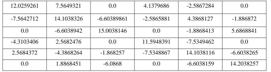
Table 3 Approximated values of Jacobian elements of eq.(19) computed using Finite Differentiation (FD) method
Table 4 Accurate values of Jacobian elements of eq.(19) computed using Automatic Differentiation (AD) method
After seven iterations of convergence, it is witness from the above tables that Jacobian matrix obtained by complex and tedious Finite Differentiation method gives the approximated values of the derivatives with truncation errors as shown in table 3. Whereas the Jacobian matrix obtained using Automatic Differentiation method gives the exact and accurate values of the derivatives as shown in table 4.
12.0259261 7.5649321 0.0 4.1379686 -2.5867284 0.0
-7.5642712 14.1038326 -6.60389861 -2.5865881 4.3868127 -1.886872
0.0 -6.6038942 15.0038146 0.0 -1.8868413 5.6868841
-4.3103406 2.5682476 0.0 11.5948391 -7.5349462 0.0
2.5684372 -4.3868264 -1.868257 -7.5348867 14.1038116 -6.6038265
0.0 1.8868451 -6.0868 0.0 -6.6038159 14.2038257
12..224168 -7.5631215 0.0 4.13761684 -2.58649241 0.0
-7.5634986 14.1034467 -6.6012781 -2.5863276 4.3854144 -1.8862221
0.0 -6.6025635 15.0037971 0.0 -1.8862341 5.6821826
-4.31001899 2.5681389 0.0 11.5931551 -7.53214668 0.0
2.5682344 -4.3862126 -1.8848212 -7.532156 14.1027827 -6.6034489
Using the jacobian values obtained in table 3 and table 4 by both Finite Differentiation and Automatic Differentiation for further calculations of real power, reactive power. voltage and load angle at each bus of the given test system using the eq.(19), will contributes following final results of Newton Raphson power flow solution .
Table 5 Final Power flow solution of given 4 bus system due to the Jacobian elements obtained by the Finite Differentiation
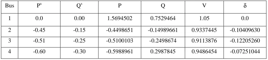
Table 6 Final Power flow solution of given 4 bus system due to the Jacobian elements obtained by the Automatic Differentiation
.
It is observed from the table 5 that ,because of the inaccurate, approximated Jacobian values obtained by Finite Differentiation shown by table 3, the final power flow solution presents unfair values of real power, reactive power, voltage, angle at each bus as shown in table 5, in contrast to this it is observed from the table 6 that , owing to the accurate Jacobian values obtained by AD shown by table 4, the final power flow solution provides accurate and noticeably improved values of real power, reactive power, voltage, angle at each bus as shown in table 6. It is also noticed from the table 6 that the power mis matches are considerably very small and almost equal to zero, due to the improved values of powers resulted from accurate values of Jacobians obtained by Automatic Differentiation.
Conclusions
A model has been formulated for a four bus power system network then the technique of Automatic Differentiation tested, implemented using that system and the effectiveness of this technique is demonstrated.
References
[1] P.Kundur, (1994). Power System Stability and Control, McGraw-Hill.
[2] Arrillaga, J. and Arnold, C.P(1990). Computer Analysis of Power Systems, John Wiley & Sons, [3] Stott(1974): Review of Load-flow Calculation Methods”, IEEE Proceedings, vol. 62, pp 916–929.
[4] Alguacil N.and J.Conejo (2000): Multiperiod optimal power flow using benders decomposition, IEEE Transactions on power systems, pp. 196-201.
[5] Da Costa V.M., N. Martins, and J.L.R., Pereira (1999): Developments in the Newton – Raphson Power flow formulation based on current injections, IEEE Transactions on power systems, pp. 1320-1326.
[6] Da CostaV.M., N. Martins, and J.L.R.Pereira (2001): An augmented Newton – Raphson Power flow formulation based on current injections, Int. J. Electrical Power and energy Systems. Vol. 23, pp. 305-312.
[7] A. Griewank(2000). Evaluating Derivatives: Principles and Techniques of Algorithmic Differentiation, Frontiers in Applied Mathematics, SIAM, Philadelphia, PA .
[8] T. F. Coleman and A.Verma(1998). ADMAT: An Automatic Differentiation Toolbox for MATLAB, Technical report, Computer Science Department, Cornell University.
[9] Richard D. Neidinger (2010): Introduction to Automatic Differentiation and MATLAB Object-Oriented Programming, SIAM REVIEW, Vol. 52, No. 3.
Bus Ps Qs P Q V δ
1 0.0 0.00 1.5694502 0.7529464 1.05 0.0
2 -0.45 -0.15 -0.4498651 -0.14989661 0.9337445 -0.10409630
3 -0.51 -0.25 -0.5100103 -0.2498674 0.9113876 -0.12205260
4 -0.60 -0.30 -0.5988961 0.2987845 0.9486454 -0.07251044
Bus Ps Qs P Q V δ
1 0 0 1.5523461 1.7516422 1.05 0.0
2 -0.45 -0.15 -0.4499982 -0.1499982 0.9323438 -0.1039961
3 -0.51 -0.25 -0.5098891 -0.2500068 0.9210649 -0.1236567