Detecting Ancient Balancing Selection: Methods And Application To Human

University of Pennsylvania

ScholarlyCommons

Publicly Accessible Penn Dissertations

2019

Detecting Ancient Balancing Selection: Methods

And Application To Human

Katherine Siewert

University of Pennsylvania, [email protected]

Follow this and additional works at:https://repository.upenn.edu/edissertations

Part of theBioinformatics Commons,Evolution Commons, and theGenetics Commons

This paper is posted at ScholarlyCommons.https://repository.upenn.edu/edissertations/3313 For more information, please [email protected].

Recommended Citation

Siewert, Katherine, "Detecting Ancient Balancing Selection: Methods And Application To Human" (2019).Publicly Accessible Penn Dissertations. 3313.

Detecting Ancient Balancing Selection: Methods And Application To

Human

Abstract

Balancing selection can maintain genetic variation in a population over long evolutionary time periods. Identifying genomic loci under this type of selection not only elucidates selective pressures and adaptations but can also help interpret common genetic variation contributing to disease. Summary statistics which capture signatures in the site frequency spectrum are frequently used to scan the genome to detect loci showing evidence of balancing selection. However, these approaches have limited power because they rely on imprecise signatures such as a general excess of heterozygosity or number of genetic variants. A second class of statistics, based on likelihoods, have higher power but are often computationally prohibitive. In addition, a majority of methods in both classes require a high-quality sequenced outgroup, which is unavailable for many species of interest. Therefore, there is a need for a well-powered and widely-applicable statistical approach to detect balancing selection. Theory suggests that long-term balancing selection will result in a genealogy with very long internal branches. In this thesis, I show that this leads to a precise signature: an excess of genetic variants at near identical allele frequencies to one another. We have developed novel summary statistics to detect this signature of balancing selection, termed the β statistics. Using simulations, we show that these statistics are not only computationally light but also have high power even if an outgroup is unavailable. We have derived the variance of these statistics, allowing proper comparison of β values across sample sizes, mutation rates, and allele frequencies - variables not fully accounted for by many previous methods. We scanned the 1000 Genomes Project data with β to find balanced loci in humans. Here, I report multiple balanced haplotypes that are strongly linked to both association signals for complex traits and regulatory variants, indicating balancing selection may be affecting complex trait architecture. Due to their high power and wide applicability, the β statistics enable evolutionary biologists to detect targets of balancing selection in a range of species and with a degree of specificity previously unattainable.

Degree Type

Dissertation

Degree Name

Doctor of Philosophy (PhD)

Graduate Group

Genomics & Computational Biology

First Advisor

Benjamin F. Voight

Keywords

Balancing selection, Natural selection, Selection scans

Subject Categories

DETECTING ANCIENT BALANCING SELECTION: METHODS

AND APPLICATION TO HUMAN

Katherine M. Siewert

A DISSERTATION

in

Genomics and Computational Biology

Presented to the Faculties of the University of Pennsylvania

in

Partial Fulfillment of the Requirements for the

Degree of Doctor of Philosophy

2019

Supervisor of Dissertation

Benjamin F. Voight, Ph.D., Associate Professor of Systems Pharmacology and Trans-lational Therapeutics and Genetics

Graduate Group Chairperson

Benjamin F. Voight, Ph.D., Associate Professor of Systems Pharmacology and Trans-lational Therapeutics and Genetics

Dissertation Committee:

Marcella Devoto, Ph.D., Professor of Pediatrics and Epidemiology Sarah A. Tishkoff, Ph.D., Professor of Genetics and Biology Junhyong Kim, Ph.D., Professor of Biology

Acknowledgments

I am lucky enough to have a large number of people to thank for making my time

in graduate school both enjoyable and fruitful. I would first and foremost like to

thank my advisor, Ben Voight. He is in large part responsible for turning me into the

scientist I am today, both by modeling science as a process driven by excitement and

curiosity and through viewing it as a question-driven endeavor. His support, trust

and patience allowed my PhD to be a happy six years. In addition, I am grateful for

my thesis committee: Marcella Devoto, Sarah Tishkoff, Junhyong Kim and Philipp

Messer for their time and gracious advice.

I have been lucky to have been a part of the amazing group of individuals that compose

the Voight Lab. Kelsey Johnson, you deserve an especially large shout-out, as it has

been both fun and motivating working towards our PhDs together. Thank you for all

of our conversations, whether it be about science or life, as well as for the occasional

well-deserved sass when I said something truly ridiculous! Thank you to Paul Babb

for being a constant source of support and encouragement, and for being a model of

encouraging my inquisitive and outspoken nature, even to the occasional exasperation

of our poor advisor and labmates.

Kat Gawronski – I thank you for being both a close friend and an amazing support

system – conversations with you seemed to either lead to laughter, me learning

some-thing interesting, or both! Onur Y¨or¨uk, the same goes for you. I would also like to

thank Kim Lorenz, Chris Thom, and Diana Cousminer for their wise feedback and

support throughout my PhD. Finally, I would like to thank Will Bone and Chris

Adams for making my last few years of PhD full of fun discussion, both scientific and

otherwise.

I owe much to the inspiring and supportive scientific community at Penn, including

my friends, professors, administrators and colleagues. I would like to give a special

acknowledgment to the GCB students in my year: Alex Amlie-Wolf, Lucy Shan,

Salika Dunatunga, Brett Beaulieu-Jones and Ian Mellis. I could not have asked to be

a part of a more intelligent, mature and supportive group of individuals.

I also thank my family for turning me into the person I am today. I am grateful

for my parents for modeling and encouraging curiosity, critical thinking and hard

work, for which I credit my PhD to more than anything else. Gretchen Siewert, you

are a never-ending source of laughter and support! Finally, I would like to thank

my partner Jason Rocks. You’ve been my rock throughout graduate school and

DETECTING ANCIENT BALANCING SELECTION: METHODS AND

APPLICATION TO HUMAN

Katherine M. Siewert

Benjamin F. Voight, Ph.D.

Balancing selection can maintain genetic variation in a population over long

evolu-tionary time periods. Identifying genomic loci under this type of selection not only

elucidates selective pressures and adaptations but can also help interpret common

genetic variation contributing to disease. Summary statistics which capture

signa-tures in the site frequency spectrum are frequently used to scan the genome to detect

loci showing evidence of balancing selection. However, these approaches have limited

power because they rely on imprecise signatures such as a general excess of

heterozy-gosity or number of genetic variants. A second class of statistics, based on likelihoods,

have higher power but are often computationally prohibitive. In addition, a majority

of methods in both classes require a high-quality sequenced outgroup, which is

un-available for many species of interest. Therefore, there is a need for a well-powered

and widely-applicable statistical approach to detect balancing selection. Theory

sug-gests that long-term balancing selection will result in a genealogy with very long

internal branches. In this thesis, I show that this leads to a precise signature: an

excess of genetic variants at near identical allele frequencies to one another. We have

developed novel summary statistics to detect this signature of balancing selection,

computationally light but also have high power even if an outgroup is unavailable. We

have derived the variance of these statistics, allowing proper comparison of β values

across sample sizes, mutation rates, and allele frequencies - variables not fully

ac-counted for by many previous methods. We scanned the 1000 Genomes Project data

with β to find balanced loci in humans. Here, I report multiple balanced haplotypes

that are strongly linked to both association signals for complex traits and regulatory

variants, indicating balancing selection may be affecting complex trait architecture.

Due to their high power and wide applicability, the β statistics enable evolutionary

biologists to detect targets of balancing selection in a range of species and with a

Contents

1 Introduction 1

1.1 A brief history of balancing selection . . . 2

1.1.1 Development of the theory of overdominance as a source of hybrid vigor . . . 2

1.1.2 Modern definitions of balancing selection . . . 3

1.1.3 Examples of balanced loci . . . 3

1.2 The effect of balancing selection on coalescence and patterns of variation 5

1.2.1 Effects of balancing selection on the coalescent process . . . . 5

1.2.2 Effects of extended time to most recent common ancestor on the site frequency spectrum . . . 7

1.3 Detecting balancing selection: statistics and scans . . . 9

1.3.1 Motivation for detecting balancing selection . . . 9

1.3.2 Classic methods for detecting balancing selection based on the site frequency spectrum . . . 10

1.3.3 Trans-species SNPs and haplotypes as a signature of balancing selection . . . 12 1.3.4 Recent statistics to detect balancing selection: Composite

like-lihood methods . . . 14 1.3.5 Power and applicability of existing method for detecting

bal-ancing selection . . . 15

1.4 Genome-wide impact of balancing selection . . . 17

1.4.1 Debate on the importance of balancing selection to evolution . 17 1.4.2 Effects of balancing selection on the deleterious mutation load 19 1.5 Motivation for a new method for detecting ancient balancing selection 21 2 Detecting ancient balancing selection using an excess of allele fre-quency similarity 22 2.1 Effects of balancing selection on the site frequency spectrum . . . 23

2.1.1 A forward in time perspective . . . 23

2.1.2 A coalescent perspective . . . 23

2.1.3 Effects of recombination on the signature of balancing selection 25 2.2 The β(1) _{statistics for detecting balancing selection . . . . 26}

2.2.1 Framework for capturing excess allele frequency correlation . . 26

2.2.2 Capturing allele frequency correlation . . . 27

2.2.3 Choice ofp parameter . . . 28

2.2.4 Estimator of the mutation rate based on allele frequency corre-lation . . . 31

2.2.5 A summary statistic to detect balancing selection based on the site frequency spectrum . . . 32

2.2.6 Properties of β(1) _{in simulations . . . . 34}

2.2.7 On the assumption of independence between basepairs . . . . 35

2.3 Standardization of the β(1) statistics . . . 36

2.3.1 Variance of the unfolded β statistic . . . 37

2.3.2 Variance of the folded β statistic . . . 37

2.3.3 Standardized β statistics . . . 39

2.4 Window size containing signature of balancing selection . . . 40

2.5.1 Simulations . . . 42

2.5.2 Method of power comparison . . . 44

2.5.3 Power comparison results . . . 47

3 Application of β(1) _{to detect balancing selection in humans 63} 3.1 Overview of scan . . . 63

3.2 Methods for 1000 Genomes Analysis . . . 65

3.3 Characterization of signals . . . 67

3.4 A signature of balancing selection at the CADM2 locus . . . 69

3.5 A signature of balancing selection near the diabetes associated locus, WFS1 . . . 71

3.6 Discussion of top β loci . . . 72

4 Detecting ancient balancing selection using substitutions 76 4.1 Derivation of ˆθD and its variance . . . 77

4.2 Estimation of the speciation time . . . 82

4.3 Power analysis . . . 84

4.3.1 Power analysis ofβ(2) and standardized β statistics . . . 84

4.3.2 Techniques for power comparison . . . 88

4.3.3 Comparison with prior power analyses. . . 90

4.3.4 Comparison of β(2) _{and N CD2 statistics. . . . 91}

4.4 Estimation of the background mutation rate . . . 93

5 Conclusions and future directions 96 5.1 The β statistic in perspective . . . 96

5.2 Potential improvements to the β statistics . . . 98

List of Figures

1.1 Coalescent trees: balanced versus neutral . . . 7

1.2 Site frequency spectrum under balancing selection . . . 8

2.1 Cartoon of allelic class-build up . . . 24

2.2 Coalescent look at alleleic class build-up . . . 25

2.3 Simulations demonstrate allelic-class build-up . . . 26

2.4 Similarity function visualized . . . 29

2.5 Power of Beta with differentp parameter values . . . 30

2.6 β(1) _{distribution in simulations . . . . 35}

2.7 Power of conditional β statistic . . . 36

2.8 Power analysis using different window sizes . . . 43

2.9 Power ofT1 and T2 with different numbers of informative sites . . . 46

2.10 Power analysis with basic demography . . . 48

2.11 Power analysis with population expansion . . . 49

2.12 Power analysis with population bottleneck . . . 50

2.13 Power analysis with subdivided population . . . 52

2.14 Power analysis with introgression . . . 55

2.16 Power analysis with low mutation rate . . . 57

2.17 Power analysis with high recombination rate . . . 58

2.18 Power analysis with low recombination rate . . . 59

2.19 Power analysis by sample size, younger selection . . . 60

2.20 Power analysis by sample size, older selection . . . 60

2.21 Power of β(1) _{with sub-sampling of individuals across values of p . . . 61}

2.22 Power analysis with frequency-dependent selection . . . 62

2.23 Power analysis with weak selection . . . 62

3.1 β(1) _{distribution in 1000 Genomes populations . . . . 64}

3.2 Signal of balancing selection atCADM2 . . . 68

3.3 Signal of balancing selection atWFS1 . . . 70

4.1 Segments of coalescent tree . . . 78

4.2 Distribution of ˆθ statistics in simulations . . . 82

4.3 Distribution of β statistics in simulations . . . 83

4.4 Power ofβ(2) _{if speciation time is incorrect . . . . 84}

4.5 Power comparison at a 1% false positive rate . . . 85

4.6 Power ofβ(2) _{compared to other methods . . . . 86}

4.7 Power ofβ(2) _{without controlling for allele frequency . . . . 87}

4.8 Power ofN CD2 statistic on different window sizes . . . 88

List of Tables

Chapter 1

Introduction

Overdominance is “due to the occurrence of a rather special class of mutations and

gene combinations, which confer on heterozygotes a higher adaptive value... Although

overdominance is, by and large, an exceptional situation, it is of particular interest

to a student of population genetics”.

1.1

A brief history of balancing selection

1.1.1

Development of the theory of overdominance as a source

of hybrid vigor

The concept of balancing selection arose from early discussions of hybrid vigor. This

phenomenon had been observed for centuries and has been of significant interest

due to its direct relevance to plant breeding (Crow, 1987). Indeed, it was noted by

Mendel, who observed that hybrid pea strains were larger and more vigorous than

parental strains (Mendel 1865). Charles Darwin also had an interest in the topic:

he wrote an entire book on inbreeding depression and hybrid vigor (Darwin, 1878).

Geneticists in the early 1900s, particularly George Shull and Edward East, suggested

that this hybrid vigor, or heterosis, was due to the increased diversity of alleles found

in an individual with higher heterozygosity. It was proposed that these alleles increase

fitness in a complementary fashion to one another (East, 1936; Shull, 1948). The term

overdominance was introduced by Fred Hull to refer to this phenomena. He defined

it as the situation in which the fitness of a heterozygote would be over the fitness

that would be observed if either allele was dominant (Hull, 1945, 1946). Although

overdominance fell out of favor as the reason for hybrid vigor (see section 1.4.1), it

1.1.2

Modern definitions of balancing selection

Throughout the next several decades, balancing selection became defined as natural

selection in which multiple alleles are maintained at a locus in a population (Levene,

1953). It can be due to overdominance as originally suggested, but further work

demonstrated that it can also be due to spatially, temporally, or negative-frequency

dependent selection. For instance, if multiple niches are present in an environment an

equilibrium can occur if alternate alleles are beneficial in the different niches (Levene,

1953; Haldane, J.B.S., Jayakar, 1963). Furthermore, if the fitness of an allele in a

population fluctuates with time, then under certain conditions, this can lead to

long-term maintenance of the alternately favored alleles (Hedricket al., 1976). Finally, the

fitness of an allele may be inversely proportional to its frequency, which will cause

the frequency of the allele to increase until it is no longer favored and has therefore

reached its equilibrium frequency (Takahata and Nei, 1990).

1.1.3

Examples of balanced loci

Throughout the last century, there has been an interest in finding genomic loci that

have experienced balancing selection. There are several classic sites long proposed

to be under this type of selection. Perhaps the most famous is the Hemoglobin-β

locus. Homozygotes for the sickle-cell allele have sickle-cell anemia, homozygotes for

the other alleles have an increased risk of malaria, while heterozygotes have resistance

2002). The major histocompatibility complex (MHC) region has also been long

hy-pothesized to be under selection for multiple reasons (Slade and McCallum, 1992).

The first is overdominance, as it could be advantageous for an immune system to be

able to respond to a wider diversity of pathogens. However, studies have shown that

the level of heterozygosity observed in the MHC in humans cannot be explained solely

by overdominance (De Boer et al., 2004). Frequency-dependent selection may be

re-sponsible for the additional signal of balancing selection in the MHC. The mechanism

for this type of selection would be that pathogens may not be adapted to overcome

rare human alleles that aid in resistance against them (Slade and McCallum, 1992).

There have also been a number of loci recently proposed to be under balancing

selec-tion with experimental or observaselec-tional evidence (Schweizer et al., 2018; Sanoet al.,

2018; Network, 2015; Wheat et al., 2010). One example is balancing selection on a

locus in North American wolves. Homozygotes and heterozygotes for the KB allele

have a black coat color, while homozygotes for the ky allele have a gray coat color

(Anderson et al., 2009). Interestingly, heterozygotes have the highest fitness in

Yel-lowstone populations, suggesting that coat color is not the only selective pressure

(Schweizer et al., 2018). Evidence suggests that overdominance may be acting at this

locus, possibly due to the K locus being involved with not only coat color, but also

immune response (Schweizer et al., 2018).

Another recently described example is spatially-dependent selection in a species of

extremophile cyanobacterium. A polymorphism which affects the function of

in this species (Fischerella thermalis) and has significantly different allele frequencies

between individuals living in two different temperatures. There is high gene flow

between the individuals living in the different temperatures, and very low population

differentiation elsewhere in the genome (Sano et al., 2018). This suggests that these

individuals are part of the same species and that this locus may be under long-term

spatially dependent selection due to adaptation to different temperature conditions.

1.2

The effect of balancing selection on coalescence

and patterns of variation

1.2.1

Effects of balancing selection on the coalescent process

Initially, a newly balanced allele will increase in frequency. This creates long

haplo-types of limited diversity, mimicking the effects of an incomplete positively selected

sweep (Charlesworth, 2006). The allele will then increase in frequency until it reaches

what is termed its equilibrium frequency – the frequency at which it is expected to

be maintained. This frequency is determined by the relative fitness of the different

genotypes. For instance, if the fitness of the two homozygote classes are equal, and

the fitness of the heterozygote is higher, then the equilibrium frequency will be 50%.

In the case of the sickle cell allele in populations in malaria-endemic regions, the

homozygotes for the sickle-cell alleles have much lower fitness than for the opposite

much lower than 50%. In malaria endemic regions estimates have found its frequency

to be no more than 18% in any population (Piel et al., 2010).

If the selective pressure is sustained, then balancing selection can maintain alleles in

populations for potentially very long time periods, given certain conditions.

Specif-ically, the selective coefficient must be high enough that the heterozygotes have a

significant fitness advantage over homozygotes (Robertson, 1962). In addition, the

equilibrium frequency must be of intermediate frequency (between about 20 and 80%)

(Takahata and Nei, 1990; Ewens and Thomson, 1970; Robertson, 1962), or genetic

drift will remove the variation after enough generations.

By maintaining polymorphism, balancing selection affects the structure of the

coa-lescent tree at the locus. Under neutrality, genetic drift will cause coalescence of all

lineages after a moderate amount of time. In contrast, neither allele can fix in the

population under balancing selection, so the time to most recent common ancestor

(TMRCA) will predate the start of balancing selection, making it potentially much

older than at a neutral locus (Fig. 1.1) (Kaplan et al., 1988). The genealogy of

each allelic class, defined as all haplotypes containing one of the two balanced alleles,

will be nearly identical to that of a neutral locus of sample size equal to the size of

the allelic class (Hey, 1991). The number of individuals in the two sub-trees is

de-termined by the equilibrium frequency. Although these characteristics will hold true

under all types of long-term balancing selection, the structure of the coalescent tree

under temporally-dependent selection may be more complex, due to the relative sizes

Figure 1.1: Balancing selection increases the time to most recent common ancestor at a locus. Circles represent haploid individuals.

1.2.2

Effects of extended time to most recent common

an-cestor on the site frequency spectrum

The long time to most recent common ancestor at a locus under balancing selection

results in old haplotypes. Due to their age, these haplotypes have had time to

accu-mulate large numbers of mutations (Charlesworth 2006). More specifically, balanced

haplotypes will accumulate their own unique alleles, but these alleles are not allowed

to fix in the population because selection constrains the frequency of the haplotype

class in which they arose (Hey, 1991). This results in the classic signature of

bal-ancing selection: an excess number of intermediate frequency alleles and a deficit of

substitutions (i.e. genomic positions in which the allele in all ingroup individuals

differs from the outgroup individual)(Fig. 1.2)(Hudsonet al., 1987; Tajima, 1989).

hap-Figure 1.2: Site frequency spectrum of derived alleles in balanced or neutral simula-tions, with core variant removed. Substitusimula-tions, i.e. positions in which the derived allele is fixed in the species under consideration, are displayed as SNPs of frequency 1.0. Window size is 500 base pairs on either side of the core site, with sample size 100 chromosomes. Based on simulations with an equilibrium frequency of 0.5.

loid two-island model (Hey, 1991). In this model, a population is split into two

isolated subpopulations. Mutations can arise on each island, but without migration

between the islands, the mutations will not reach the subpopulation on the other

island. Instead, these mutations build-up on the islands, causing an excess number

of intermediate frequency alleles when the sub-populations are combined into a site

frequency spectrum (Tajima, 1989). However, migration will allow alleles to transfer

between the two islands, reducing the number of unique alleles. Analogously,

un-der balancing selection, two haplotype classes are maintained in the population with

neither one allowed to fix due to selection. Mutations unique to each allelic class

mutations from the effects of selection (Hudson and Kaplan, 1988; Hey, 1991).

1.3

Detecting balancing selection: statistics and

scans

1.3.1

Motivation for detecting balancing selection

A number of fundamental questions in evolutionary biology can be addressed through

scans for natural selection. One key question is what selective pressures species have

experienced throughout their evolutionary history, and how they have adapted to

these pressures. If a balanced locus is detected in a scan for selection, then

compu-tational and/or experimental approaches may be used to figure out what phenotypes

the locus is associated with. In some cases, the causal selective pressures on the

locus can be inferred. This process has successfully uncovered multiple targets of

balancing selection and their associated phenotypes, as discussed in section 1.1.3,

though I note that only some of these began with a genome-wide scan for selection.

Scans for positive selection and follow-up have been more successful, possibly owing

to a larger history of methodological development for detecting positive selection.

Established sites under positive selection in humans with an established phenotype

include EDAR for hair follicle thickness (Kamberov et al., 2013), lactase persistence

(Bersaglieri et al., 2004; Tishkoff et al., 2007), alcohol dehydrogenase (Osier et al.,

et al., 2018). These successes in scans for positive selection bode well for the goal of

detecting and explaining sties under balancing selection.

In fact, one advantage of detecting balancing selection is that it leaves a much

nar-rower footprint in the genome than does positive selection (Section 2.4). This results

in a smaller number of possible causal variants, making the identification of the true

causal variant easier. Despite this factor, the number of balanced loci in humans

with an established phenotype and/or selective pressure is very limited, motivating

the need research on balancing selection.

A second key question scans for selection can help answer is the impact different types

of selection have had on patterns of variation in species. This is discussed more in

section 1.4. In short, in order to identify the prevalence of balancing selection, we

must first develop a better understanding of its effects on genomic loci under this

type of selection.

In order to answer both these questions, a highly specific signature of balancing

selection, and a corresponding high-powered test for its detection, is needed.

1.3.2

Classic methods for detecting balancing selection based

on the site frequency spectrum

By scanning population-level sequencing data for the signatures of selection, loci

meth-ods of doing so calculate a statistic sensitive to the effects of balancing selection on

the site frequency spectrum in a sliding window across the genome.

Tajima’s D is one such statistic. It is the difference of two unbiased estimators

of the mutation rate. Intuitively, these estimators estimate the mutation rate by

counting the number of SNPs, using the intuition that a higher mutation rate will

result in a higher number of mutations in a window. Accordingly, estimators of

the mutation rate will be higher if there are more SNPs. The first estimator which

comprises Tajima’sD, θπ, estimates the mutation rate using heterozygosity. Because

the number of intermediate frequency mutations on old haplotypes is expected to be

higher than on newer haplotypes (Fig. 1.2), this estimator will increase in windows

which have experienced long-term balancing selection. The second estimator, θW,

uses the total number of SNPs in a window to estimate the mutation rate. This

estimator is relatively insensitive to balancing selection and is used to correct for

the background mutation rate. Tajima’s D is the difference of these two estimators

divided by the standard deviation (Tajima, 1989):

D= θπ−θW

V ar[θπ−θW]

(1.3.1)

Therefore, values of D significantly above zero indicate potential long-term balancing

selection, while values close to zero indicate an absence of evidence of balancing

selection.

look at allele frequencies, but instead compares only the number of polymorphisms

and the number of substitutions to their expected number under neutrality. By

com-bining these terms in a chi-squared statistic, significant deviation from neutrality can

be detected (Hudson et al., 1987). Specifically, a higher number of polymorphisms,

and a lower number of substitutions are expected under balancing selection, as

pre-viously discussed.

Several other statistical tests have also been used to detect these signatures of

bal-ancing selection. The Mann-Whitney U test can be used to detect an excess number

of intermediate-frequency alleles. This test can be used in combination with a

mod-ified HKA test, which detects an excess number of variants at a locus. The union

of these tests produced a set of loci with both higher-frequency SNPs and a higher

total number of SNPs than the background levels in the human genome, indicating

balancing selection (Andres et al., 2009).

1.3.3

Trans-species SNPs and haplotypes as a signature of

balancing selection

An orthogonal signature of balancing selection is shared SNPs or haplotypes between

multiple species. Trans-species haplotypes are defined as two or more variants that are

found in tight linkage disequilibrium and are shared between humans and a primate

outgroup (in our case, chimpanzee). If a neutral SNP was present in a common

the population in one or both species, leading to a substitution. In contrast, if the

SNP is under balancing selection in both species, it can be maintained from the time

it arose until present (Takahata, 1990; Takahata and Nei, 1990). This leads to the

segregation of both alleles in both species. Therefore, if two species share one SNP

(a trans-species SNP) or more than one SNP at a locus (a trans-species haplotype),

this indicates potential balancing selection.

The presence of trans-species SNPs may be due to recurrent mutations (i.e. the same

mutation occurs in both species independently), so are not a test for selection with

high specificity. In contrast, due to the very low probability of two recurrent

muta-tions occurring in high linkage disequilibrium under human and chimp demography

(Gao et al., 2014), trans-species haplotypes are a very specific signature of

balanc-ing selection in humans. Multiple studies have used human and chimp sequencbalanc-ing

data to detect these shared SNPs and haplotypes (Leffler et al., 2013; Teixeira et al.,

2015). These scans have identified a number of balanced loci potentially involved

in immunity, including loci involved with recognizing plasmodium falciparum (Leffler

et al., 2013) or a missense change in LAD1, an autoantigen which causes linear IgA

disease (Teixeira et al., 2015). In addition, the ABO blood group has been proposed

to be under long-term balancing selection in humans on the basis of trans-species

1.3.4

Recent statistics to detect balancing selection:

Com-posite likelihood methods

An ideal statistic to detect balancing selection would be a full likelihood estimation of

a locus being under balancing selection as opposed to being neutral. Such a statistic

could be based on summary level information about the site frequency spectrum,

such as the probability of seeing a mutation at each frequency at each distance from

a balanced SNP. Alternatively, it could make use of individual-level genotype data,

calculating the likelihood of the observed haplotype structures at various distances

from the balanced SNP. These are in contrast to the early statistics designed to detect

balancing selection, which do not rely on likelihoods and instead use a summary

statistic to capture the general patterns caused by selection.

Recently, two composite likelihood methods were developed to detect balancing

se-lection (DeGiorgio et al., 2014) which utilize the site frequency spectrum. These

statistics are composite in that they consider each SNP independently of the other

SNPs at the locus. The Kaplan-Darden-Hudson model, which describes the genealogy

of a neutral SNP linked to a selected SNP (Kaplanet al., 1988; Hudson and Kaplan,

1988), is used to model the probability of seeing a segregating site or substitution

at each recombination-scaled distance from a balanced SNP. The background levels

of polymorphism and substitutions are used to generate the expected site frequency

spectrum near a SNP evolving neutrally. By comparing these two composite

likeli-hoods, a test for balancing selection, T1, is derived (DeGiorgio et al., 2014). The T1

consider allele frequencies.

DeGiorgio et al. then derive the T2 statistic, which does take into account allele

frequencies (DeGiorgio et al., 2014). However, because the site frequency spectrum

under balancing selection is unknown, simulations are used to generate

probabili-ties of seeing SNPs at various frequencies. These simulations are performed under

specified parameter values, including a large range of equilibrium frequencies and

recombination rates. By using simulations matched for equilibrium frequency and

re-combination rate at a locus, these simulation-generated likelihoods are incorporated

into a composite likelihood framework.

1.3.5

Power and applicability of existing method for

detect-ing balancdetect-ing selection

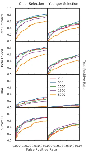
Using simulations, DeGiorgio et al. (2014) demonstrated that the power of their

T1 and T2 statistics are higher than the HKA test and Tajimas D. The power of

their T2 method is higher than T1, as would be expected because it considers allele

frequencies. However, T2 presents challenges in its applicability. Namely T2, like

the T1 and HKA test, requires an outgroup with which to call substitutions and

ancestral/derived allele states. In addition, prior to scanning the genome with the

T2 test, large numbers of simulations must be performed to generate expected site

frequency spectra. These simulations are computationally intensive, making wide

In some cases, a sequenced individual from an outgroup species is unavailable,

render-ing all these summary statistics inapplicable except Tajima’s D. However, Tajima’s

D has the lowest power to detect balancing selection in the analysis of DeGiorgio

et al. (2014). Furthermore, calling trans-species SNPs and trans-species haplotypes

requires multiple outgroup individuals. This suggests the need for new methods to

detect selection which do not require an outgroup but have the high power of theT2

method.

1.3.6

Coalescent methods

Recent methods seek to directly estimate the time to most recent common ancestor

(TMRCA), as opposed to using summary statistics. These methods are based on the

pairwise sequentially Markovian coalescent (PSMC) method (Li and Durbin, 2011).

This method models coalescent times between two individuals at a locus along the

genome using a hidden Markov model, with the hidden state being the TMRCA, and

emissions being whether the two haploid individuals match (produce a homozygote)

or have different alleles (produce a heterozygote). Transitions between states are the

result of recombination. The longer the coalescence time between the individual, the

more time there has been for mutations to build-up between them. Therefore, the

number of heterozygote sites will be proportional to the TMRCA of the individuals

at the locus. Specifically, the number of SNPs occurring on a branch is exponentially

lengths.

More recent methods have adapted the PSMC method to multiple genomes. One

such method, ARGweaver, was used to detect loci with extremely old TMRCAs,

indicative of balancing selection (Rasmussen et al., 2014). However, these methods

are computationally intensive, taking multiple days to weeks to estimate

genome-wide TMRCAs on a high-powered computer. Recent methods have continued to

improve on these methods, both in terms of speed and applicability, however, they

remain prohibitively computationally expensive for general use (Palamaraet al., 2018;

Speidel et al., 2019).

1.4

Genome-wide impact of balancing selection

1.4.1

Debate on the importance of balancing selection to

evo-lution

Since its conception, there has been an unanswered question about prevalence of

bal-ancing selection in the evolutionary history of both humans and other species. In the

early to mid 1900s, there was a debate as to why the increased number of

heterozy-gotes seen in hybrid individuals increases vigor. Many argued it was due to there

being less recessive deleterious alleles in the homozygote state in hybrids, termed

the dominance hypothesis (Bruce, 1910). Others favored the idea that it was due to

mutations in populations than would be expected, as would be expected due to long

term balancing selection (Crow, 1998). However, the overdominance explanation fell

out of favor, as it became clear that the mutation rate was higher than previously

thought and that some of the observed overdominance was due to deleterious

reces-sive alleles being linked to vigor-increasing dominant alleles (Moll et al., 1963). In

addition, experimental evidence showed that the dominance hypothesis better fit the

fitness patterns seen with various genetic crosses (Crow, 1998).

However, despite the general consensus that overdominance was not as widespread

as previously thought, the field still lacked an understanding of exactly how rare it

was. The availability of genome sequencing from humans and other primates allowed

a reconsideration of the debate decades later. An early scan for trans-SNPs using

expressed sequence tags and virtual transcripts found little evidence of trans-species

SNPs between human and chimpanzee (Asthana et al., 2005). A year later, a scan

for high polymorphism density found no loci showing significant evidence of ancient

balancing selection (Bubb et al., 2006).

However, more recent datasets, which contain whole-genome, high-quality genetic

variation data, enable a more comprehensive look into the prevalence of ancient

balancing selection. Multiple recent papers have looked for shared haplotypes

be-tween human and one or more primate outgroups and have found a number of shared

haplotypes. Leffler et al. (2013) found 125 shared haplotypes between human and

chimpanzee. A more recent paper looked for trans-species SNPs shared between

very conservative filters (Teixeira et al., 2015)

These trans-species SNPs and haplotypes are potentially only a small number of the

total balanced loci in the genome. This is because for a balanced locus to be

trans-species, the balancing selection must predate speciation, and the balanced haplotypes

must not have drifted out of the population in either species, which could occur either

because of a change in selective pressures or demography encouraging loss of variation.

Therefore, the presence of trans-species SNPs and haplotypes in the genome indicate

that balancing selection may have played a larger role in the evolution of humans than

previously thought. However, the extent to which balancing selection has shaped

patterns of variation in humans remains an open debate (Hedrick, 2012; Key et al.,

2014).

1.4.2

Effects of balancing selection on the deleterious

muta-tion load

One might predict that deleterious mutation which occur in a species will be quickly

removed by purifying selection. Therefore the number of deleterious mutations should

be low, and any deleterious mutations that do segregate should be of recent origin and

at low frequency. In contrast to this expectation, it has been suggested that there is

an excess number of intermediate frequency deleterious mutations segregating in the

human genome, termed the deleterious mutation load (Hennet al., 2015). One reason

effective (Keinan and Clark, 2012; Eyre-Walker and Keightley, 1999). However, there

is ongoing debate as to how much of the deleterious mutation load can be credited to

human demography (Doet al., 2015; Simons et al., 2014).

An alternative explanation for the deleterious mutation load in humans is balancing

selection, which can increase the deleterious mutation load via multiple mechanisms.

The first is that the deleterious mutation can be the direct target of balancing

se-lection, as is the case with the sickle cell allele at the human hemoglobin-β locus

(Allison, 1954). The second is that the deleterious mutation can be on the same

haplotype as the sweeping allele upon the start of balancing selection. The

delete-rious mutation will be swept up to intermediate frequency along with the balanced

haplotype and will be maintained in the population until being decoupled from the

balancing selection due to recombination. It has been proposed that this mechanism

is responsible for some fraction of the deleterious mutations in the MHC region (Lenz

et al., 2016). Therefore, if balancing selection is common throughout the genome, it

could be partly responsible for the deleterious mutation load in humans.

By increasing the number and frequency of deleterious variants, balancing selection

may raise the heritability of complex traits by increasing the variance in the trait

explained by genetics. This leads to the untested hypothesis that balanced loci may

have increased trait heritability. Furthermore, if this hypothesis is true, then balanced

loci should be prioritized in scans for disease-causing loci, as they have a higher

1.5

Motivation for a new method for detecting

an-cient balancing selection

In summary, understanding where balancing selection has acted on the genome is

of interest for multiple reasons: (1) it can reveal selective pressures, (2) adaptations

to those pressures, (3) identify loci which may be influencing risk for disease and

(4) help explain the deleterious mutation load. However, high power and

widely-applicable methods for detecting balancing selection are critical to answer all four of

these questions. As discussed in section 1.3, prior to this thesis, methods to detect

this type of selection suffered from at least one of the following drawbacks: (1) They

were of lower power, (2) they required an outgroup sequence or (3) they were too

computationally intensive for wide applicability. It is the aim of this thesis to develop

Chapter 2

Detecting ancient balancing

selection using an excess of allele

frequency similarity

The results of this chapter are presented in:

Siewert, K.M. and Voight B.F. 2017. Detecting Long-Term Balancing Selection Using

2.1

Effects of balancing selection on the site

fre-quency spectrum

2.1.1

A forward in time perspective

Consider a new neutral mutation that arises within an outcrossing, diploid population.

In a genomic region not experiencing selection, this mutation is expected to eventually

either drift out of the population, or become fixed (i.e., become a substitution).

However, if the SNP is under balancing selection, then the allele’s frequency can reach

no higher than the frequency of the balanced allele it arose in linkage with, assuming

no recombination. This is because the frequency is constrained by selection. Without

a recombination event and given enough time, variants that are fixed within these

allelic classes (defined by the selected variant) accumulate (Fig. 2.1). In addition

to this build-up of variants, there will be a corresponding reduction in the number

of substitutions, because the variants that may have fixed in the population without

balancing selection can instead reach a frequency no higher than that of the balanced

allele that they are linked to.

2.1.2

A coalescent perspective

As discussed prior (Section 1.2), balancing selection causes long internal branches on

a locus’s coalescent tree. These internal branches will be ancestral to all sampled

New Balanced SNP Arises

Balanced SNP Reaches Equilibrium Frequency

Fixation of Variation within Allelic Class

After Recombination

Figure 2.1: Model of allelic class build-up. (1) A new SNP (red star) arises in the population and is subject to balancing selection. (2) It sweeps up to its equilibrium frequency. (3) New SNPs enter the population linked to one of the two balanced alleles and some drift up in frequency. However, unlike in the neutral case, their maximum frequency is that of the balanced allele they are linked to, so variants build-up at this frequency (e.g., blue diamond or brown circle). (4) Recombination decouples SNPs (e.g., purple pentagon) from the balanced site, allowing them to experience further genetic drift.

class. Therefore, mutations occurring on these branches will be fixed within their

allelic class (i.e. at the frequency of the balanced allele that they are linked to)

(Fig. 2.2). This contrasts with a tree representing a neutral locus, in which all

lineages will have coalesced more recently. Any mutations occurring on the tree after

(going backwards in time) this coalescent event will have occurred in an ancestor

to all individuals at this locus and will therefore be a substitution when the locus

is compared to an outgroup species. Therefore, once again, our model of balancing

selection predicts that under balancing selection there will be an excess number of

variants at identical frequency to the balanced alleles and a deficit of substitutions,

Figure 2.2: Long internal branches cause build-up of alleles at identical frequencies under balancing selection. Branches are colored by allelic class, which here have frequencies 3/5 (blue) and 2/5 (red).

2.1.3

Effects of recombination on the signature of balancing

selection

Eventually, recombination decouples variants from the balanced allele, which allows

them to drift to loss or fixation within the population (Fig. 2.1). However, even

after recombination, the frequency of the genetic variants previously fixed in their

allelic class will remain close to that of their previous class until enough time has

passed for genetic drift to significantly change their frequencies. In our simulations

of balancing selection, a window expected to have experienced recombination since

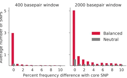
selection’s start still has an excess number of variants at similar frequencies to the

balanced variant. However, there is a smaller excess at identical frequencies relative

Figure 2.3: Simulations demonstrate the build-up of alleles at frequencies similar to balanced alleles as compared with selectively neutral counterparts. The 400 basepair window is not expected to have experienced recombination between allelic classes since the start of selection, whereas the 2000 basepair window is more likely to have.

2.2

The

β

statistics for detecting balancing

se-lection

2.2.1

Framework for capturing excess allele frequency

corre-lation

To detect loci under ancient balancing selection we therefore want to develop a

sum-mary statistic which captures an excess number of SNPs at near identical frequencies

to one another. We will use several components to do this. The first is a measure

of allele frequency similarity. This allows one to weight SNP counts based on their

into an estimator of a mutation rate. Finally, we use this estimator in combination

with another estimator that measures the background mutation rate as our statistic.

In addition, we derive the variance of this statistic, so we can standardize it.

In this chapter I present two versions of this statistic. The first, the unfolded version,

takes into account the ancestral/derived state at each SNP. By doing so, it can give

more weight to SNPs of higher frequency, because they are less likely under neutrality.

The second version, the folded version, does not use allele ancestral/derived states.

Therefore, it is applicable even to species without a high-quality sequenced outgroup

species.

2.2.2

Capturing allele frequency correlation

To capture allele frequency correlation, we derive a measurement of frequency

simi-larity between a core variant and a second variant of interest. Let n be the number

of chromosomes sampled,f0 be frequency of the core SNP, fi be the frequency of the

second SNP, i, and p be the scaling constant. Finally, g(f) returns the folded allele

frequency and m is the maximum possible folded allele frequency difference between

the core SNP and SNP i, We then measure the similarity in frequency, di, by:

g(f) = min(f, n−f) (2.2.1)

m= maxg(f0), n

2 −g(f0)

(2.2.2)

di =

1− |g(f0)−g(fi)| m

p

Thus, g(f0)−g(fi) is the folded frequency difference between the core SNP and the

SNP under consideration. We then divide by m, the maximum folded frequency

difference possible with the core SNP, to get the percent of the maximum frequency

different the two SNPs have. We then take 1 minus the result to give a similarity

metric instead of a distance metric. We raise it to the power pso that we can weight

variants in a non-linear fashion with respect to this fraction. Therefore,di can range

from 0 if a SNP has the maximum frequency difference with the core SNP, to 1 if

SNP i is at the same frequency as the core SNP (Fig. 2.4). Guidance on the

choice of p is given in section 2.2.3. We use the folded site frequency spectrum in

calculating di, as the frequency difference between the core variant and the second

variant is independent of whether the derived or ancestral allele of the nearby allele

is in linkage with the derived or ancestral core allele.

In a region under long-term balancing selection, the average di between a core SNP

and the surrounding variants is expected to be elevated. However, di alone is not

op-timally powered to detect balancing selection, as its value will be sensitive to changes

in the mutation rate in the surrounding region, and it does not take into account the

probability of seeing each allele frequency under neutrality.

2.2.3

Choice of

p

parameter

The power of our method lies in capturing allele frequency correlations. The

Figure 2.4: Absolute value of allele frequency similarity with core SNP (|g(f0)−g(fi)|) versus allele frequency similarity (di) as used by the β statistics, by different values of the p parameter. The grey and red lines represent the value of di at the given frequency similarity, while the light red bars represent the number of SNPs at a given frequency difference away from the core SNP in simulations of balancing selection, based on the 2000 basepair window panel of Fig. 2.3.

approaches infinity, the only sites that contribute towards θB are those that exactly

match the frequency of the core SNP. Atp= 0, all SNPs contribute the same amount

to the estimate of ˆθB, and so ˆθB becomes equivalent to ˆθw. Simulations show that

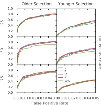
our method is fairly robust to choice of p (Fig. 2.5).

That said, the optimal p will depend on the data set at hand. If allele frequency

estimates are known to be inaccurate or sample sizes vary between SNPs, then a lower

p may be more optimal, because variants fixed in allelic class may not accurately be

called as being at identical frequency to the core SNP. In addition, by including SNPs

at very similar frequency to the core SNP in the calculation of ˆθB, SNPs that were

once fixed in class, but are no longer due to recombination followed by a small amount

of drift, are included. However, makingp too low will result in the inclusion of allele

0.0 0.2 0.4 0.6 0.8 1.0 .2 5

Older Selection

Younger Selection

0.0 0.2 0.4 0.6 0.8 .5 0

0.00 0.01 0.02 0.03 0.04 0.0 0.2 0.4 0.6 0.8 .7 5

0.00 0.01 0.02 0.03 0.04 0.05 1

2 10 20 1000

False Positive Rate

Tr

ue

P

os

itiv

e R

at

e

In this chapter, we chose a p = 20, which gives the most weight to exact frequency

matches, and a small amount of weight to very near, but not exact frequencies. If

varying sample sizes are used for each SNP, then a lower p value may be optimal

(Fig. 2.21).

2.2.4

Estimator of the mutation rate based on allele

fre-quency correlation

Derivation of Unfolded θB

Let n be the number of chromosomes sampled, di be the similarity measure and Si

be the number of variants at frequencyi in the sample.

E[

n−1

X

i=1

idiSi] =

n−1

X

i=1

E[idiSi] (2.2.4)

=

n−1

X

i=1

idiE[Si] (2.2.5)

=

n−1

X

i=1

idi 1

iθ (2.2.6)

ˆ

θβ =

n−1

P

i=1

idiSi

n−1

P

i=1

di

Derivation of Folded θB

E[

n−1

X

i=1

diSi] =

n−1

X

i=1

E[diSi] (2.2.8)

=

n−1

X

i=1

diE[Si] (2.2.9)

=

n−1

X

i=1

di 1

iθ (2.2.10)

ˆ

θ=

n−1

P

i=1

diSi

n−1

P

i=1

di1_i

(2.2.11)

Let g(x) be the folded frequency of a SNP of frequency x, Sg(x) be the number of

SNPs at that folded frequency, h=.5(n−1) andm=.5n. Folding the site frequency

spectrum, we obtain:

ˆ

θ∗_β =

Pm

i=1diSg(i)

Pm

i=1di(

1

i +

1

n−i)

1 1+δi,n−i

(2.2.12)

2.2.5

A summary statistic to detect balancing selection based

on the site frequency spectrum

We propose a statistic, β, that uses our measure of allele frequency correlation, di,

incorporated in θβ, combined with a measure of the overall mutation rate, to detect

balancing selection. Our approach is inspired by previous summary statistics of the

the difference between two estimators of θ, the population mutation rate parameter,

one of which is more sensitive to characteristics of the site frequency spectrum

dis-torted in the presence of natural selection. We propose to calculate β at each SNP

in a region of interest to identify loci in which there is an excess of variants near the

core SNP’s allele frequency, as evidence of balancing selection.

It has been previously shown that the mutation rate in a region can be estimated

as: ˆθi =Si∗i, where Si is the total number of derived variants found i times in the

window from a sample ofn chromosomes in the population (Fu, 1995). An estimator

of θ can then be obtained by taking a weighted average of θi. In our method, we

weight by the similarity in allele frequency to the core SNP, as measured by di. If

there is an excess of variants at frequencies close to the core SNP allele frequency,

then our new estimator, θβ, will be elevated. We propose:

β(1) = ˆθβ−θˆw (2.2.13)

β(1)∗ = ˆθ∗_β−θˆw (2.2.14)

θw is simply Watterson’s estimator (Watterson, 1975). β is, in effect, a weighted sum

of SNP counts based on their frequency similarity to the core SNP. We exclude the

core site from our estimation of θw and θβ.

Under neutrality, the expected value of β is zero, because it is a difference of two

will be an excess number of SNPs at near identical frequencies to one another elevating

θβ substantially over the true mutation rate in the window, whileθW will be elevated

only slightly. Therefore, values of β significantly above zero are suggestive of

long-term balancing selection.

2.2.6

Properties of

β

in simulations

To better understand the properties ofβ, we used simulations (for details see section

2.5.1) to examine its distribution with and without a balanced SNP.

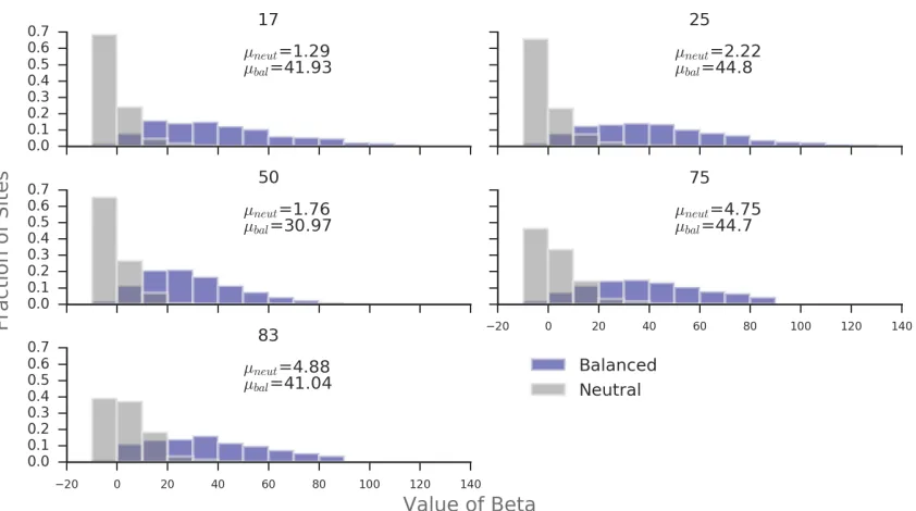
As expected, under long-term balancing selection β tends to be greater than 0, and

under neutrality it tends to be close, but slightly higher than, 0 (Fig. 2.6). Under

neutrality it is not exactly zero, because all the neutral windows β is actually

calcu-lated on will have at least one SNP, and the site frequency spectrum conditioned on

seeing a SNP of a certain frequency does not equal the unconditional site frequency

spectrum, as discussed in section 2.2.7 (Ferretti et al., 2018).

We note that the mean value of β in our neutral simulations generally increases

slightly with higher equilibrium frequencies. This behavior is expected because higher

frequency alleles will tend to have a longer TMRCA and therefore higher diversity.

The exception to this trend is neutral SNPs of frequency 0.5, which we posit is due

to the fact that this allele frequency requires the most time for mutations to drift up

Figure 2.6: Distribution of β(1) in 1kb windows around a core SNP at different equi-librium frequencies. Based on simulations using default parameters. µ refers to the mean value of β(1) _{in balanced or neutral simulations.}

2.2.7

On the assumption of independence between basepairs

In our derivations of ˆθβ we do not use the conditional site frequency spectrum. In

other words, the formula we use for the expected value and variance in SNP counts

does not take into account the frequency of the core site. However, the conditional

and unconditional SFS are unequal, as conditioning on the core SNP’s frequency gives

some knowledge about which underlying tree structures are most likely. Recently, two

papers deriving the moments of the conditional SFS were published (Ferretti et al.,

2018; Klassmann and Ferretti, 2018). We used these moments to derive a modified ˆθβ

and ˆθW conditioned on the core SNP being at the observed frequency. However, doing

so decreased power (Fig. 2.7). We posit that this is because under the conditional

0.0 0.2 0.4 0.6 0.8 1.0

False Positive Rate

0.0 0.2 0.4 0.6 0.8 1.0

Tr

ue

P

os

it

iv

e

R

at

e

β(1) _{Conditional β}(1)

Figure 2.7: Power ofβ(1) statistic when derived using the unconditional site frequency spectrum of Fu (1995) versus conditional of Ferretti et al. (2018).

core SNP is increased. Therefore, when an estimator of the mutation rate is derived

using this expected value, each SNP at that frequency is weighted less than if using

an unconditional site frequency spectrum. This behavior is opposite the ideal: we

want to give the most weight to SNPs at identical frequency to the core SNP, not

less. Therefore, the power of this statistic is reduced, so we use moments of the

unconditional site frequency spectrum to derive our β statistics and their variances.

2.3

Standardization of the

β

statistics

We next derive the variance of our statistics, enabling normalization ofβ. This allows

distribution, including population size, survey sample size, equilibrium frequencies,

and mutation rate. This is a feature lacking from other summary statistics, with the

exception of Tajima’s D (Tajima, 1989).

2.3.1

Variance of the unfolded

β

statistic

The V ar[ˆθβ] can be obtained from the formula for variance of a general group of

estimators presented in (Achaz, 2009) for which ˆθβ is a member. σ is defined in

Achaz (2009) anddi is the measure of frequency similarity presented in section 2.2.2.

V ar[ˆθβ] =

_Xn−1

i=1

di

−2

θ

n−1

X

i=1

d2_ii+θ2

n−1

X

i=1

d2_ii2σii+ 2

n−1

X

i=1

n−1

X

j=i+1

ijdidjσij

!

(2.3.1)

2.3.2

Variance of the folded

β

statistic

The formulation for β(1)∗ _{does not fall into the class of neutrality tests based on the}

folded site frequency spectrum studied in Achaz (2009), because the folded frequency

of each SNP is not considered in our formulation. Therefore, we provide a derivation

below. φ and ρ are defined in Achaz (2009) and di is the measure of frequency

sim-ilarity. Sg(i) is the number of SNPs in the window of folded frequency g(i) and is

analogous toηi in Achaz (2009). Set m=dn₂e, wherededenotes the ceiling. We refer

of β(1)∗ _is:

V ar[ˆθ_β∗ −θˆW] =V ar[ˆθβ∗] +V ar[ˆθW]−2Cov[ˆθ∗β,θˆW] (2.3.2)

First, we derive the variance of ˆθ_β∗ to be:

V ar[ˆθ∗_β] =V ar

" _Pm

i=1diSg(i)

Pm

i=1di(

1

i +

1

n−i)

1 1+δi,n−i

# = m X i=1 di 1 i + 1

n−i

1

1 +δi,n−i

!−2

V ar

" _m X

i=1

diSg(i)

# = m X i=1 di 1 i + 1

n−i

1

1 +δi,n−i

!−2 _m

X

i=1

V ar[diSg(i)] +

X

i6=j

Cov[diSg(i)djSg(j)]

! = m X i=1 di 1 i + 1

n−i

1

1 +δi,n−i

!−2 _m

X

i=1

d2_i(φiθ+ρiiθ2) +

X

i6=j

didjρijθ2

! = m X i=1 di 1 i + 1

n−i

1

1 +δi,n−i

!−2 _m

X

i=1

d2_i(φiθ+ρiiθ2) + 2

X

1≤i≤j≤m

didjρijθ2

!

(2.3.3)

Next, the V ar[ˆθW] is taken from Achaz (2009):

V ar[ˆθW] =

_Xm

i=1

n

i(n−i)(1 +δi,n−i)

−2 θ m X i=1 n

i(n−i)(1 +δi,n−i)

2

φ−_i 1

+θ2

m

X

i=1

n

i(n−i)(1 +δi,n−i)

2

φ−_i 2ρii

+ 2 m X i=1 m X

j=i+1

φ−_i 1φ−_j1 n

i(n−i)(1 +δi,n−i)

n

j(n−j)(1 +δj,n−j)

ρij

!

Finally, the covariance of ˆθ_β∗ and ˆθW:

Cov[ˆθ_β∗,θˆW] =Cov

"

Pm

i=1diSg(i)

Pm

i=1di(1_i +_n1_−i)_1+δ1_i,n−i

,

Pm

i=1Sg(i)

Pm

i=1(

1

i +

1

n−i)

1 1+δi,n−i

#

= _Pm 1

i=1di(1_i +_n1_−i)_1+δ1_i,n−i

1

Pm

i=1(

1

i +

1

n−i)

1 1+δi,n−i

Covh

m

X

i=1

diSg(i),

m

X

i=1

Sg(i)

i

= _Pm 1

i=1di(1_i +_n1−i)

1 1+δi,n−i

1

Pm

i=1(

1

i +

1

n−i)

1 1+δi,n−i

m X i=1 m X j=1

diCov[Sg(i), Sg(i)]

= _Pm 1

i=1di(1_i +_n1_−i)_1+δ1_i,n−i

1

Pm

i=1(

1

i +

1

n−i)

1 1+δi,n−i

m X i=1 m X j=1

diρijθ2

(2.3.5)

2.3.3

Standardized

β

statistics

The standardized β(1) _{statistics are given by:}

β_std(1) = β

(1)

p

V ar[β(1)_] =

ˆ

θβ −θˆW

q

α∗

nθˆ+βn∗θˆ2

(2.3.6)

β_std(1)∗ = β

(1)∗

p

V ar[β(1)∗_] =

ˆ

θ_β∗ −θˆW

q

V ar[ˆθ∗

β] +V ar[ˆθW]−2Cov[ˆθβ∗,θˆW]

2.4

Window size containing signature of balancing

selection

Although β can be calculated on any window size, previous work has suggested that

the effects of balancing selection are localized to a narrow region surrounding the

balanced site (Gaoet al., 2014). Ultimately, the optimal window size depends on the

recombination rate, as it breaks up alleleic classes.

If one uses too small of window size, then some of the signal of alleleic-class build

up will be excluded from the statistic, reducing power. It too large of window size

is used, then noise from regions beyond those which provide any signal of selection

will decrease power. Optimally, we could calculate β on the window which has not

experienced much, if any, recombination between alleleic classes. According to our

model, this region will contain all variants fixed in alleleic class, and potentially some

variants which were once fixed in alleleic class but have drifted slightly in frequency

due to recombination beginning to decouple them from selection.

The probability of recombination between allelic classes is equal to the total coalescent

branch length in the allelic class multiplied by the probability of recombination onto

the other allelic class. Because we are detecting long-term selection, most of the

coalescent branch length will fall into the portion between coalescence within each

allelic class and coalescence of the two allelic classes. We can, therefore, put an upper

bound on the size of the ancestral region. The probability of any recombination event