Machine learning as a tool for classifying electron tomographic reconstructions

(1)

R E S E A R C H

Open Access

Machine learning as a tool for classifying

electron tomographic reconstructions

Lech Staniewicz

*

and Paul A. Midgley

Abstract

Electron tomographic reconstructions often contain artefacts from sources such as noise in the projections and a “missing wedge” of projection angles which can hamper quantitative analysis. We present a machine-learning approach using freely available software for analysing imperfect reconstructions to be used in place of the more traditional thresholding based on grey-level technique and show that a properly trained image classifier can achieve manual levels of accuracy even on heavily artefacted data, though if multiple reconstructions are being processed, a separate classifier will need to be trained on each reconstruction for maximum accuracy.

Keywords: Electron tomography, Image processing, Machine learning, Image classification, Thresholding

Background

Electron tomography is a procedure carried out using a (scanning) transmission electron microscope, or (S)TEM, where, conventionally, a sample is rotated about an axis perpendicular to the electron beam and images (“projec-tions”) taken at each tilt angle (collectively known as a “tilt series”). These projections are then reconstructed into a full 3D volume of the sample [1–5], known as a tomogram. Tomography is carried out when three-dimensional information is explicitly necessary—for instance, when visualising the distribution of nanoparticles inside a poly-mer matrix [6, 7]. Quantitative 3D information (such as nearest-neighbour distances) can also be extracted from tomograms—something impossible with a two-dimensional projection of an irregular structure such as a zeolite or mesoporous catalyst [8–10].

The procedure for converting a tilt series into a full vol-ume consists of many steps, all of which can introduce error into the final result. Firstly, we consider the separate images which compose the tilt series. While every image in the series would ideally be in focus and with minimal astigmatism, this is not the case in practice—especially if using automated focus routines, low-dose techniques or simply if the sample thickness is comparable to or greater than the depth of field. Blurred images in the tilt series will

*Correspondence: [email protected]

Department of Materials Science and Metallurgy, University of Cambridge, 27 Charles Babbage Road, CB3 0FS Cambridge, UK

directly result in blurring in the final reconstruction, along with causing additional problems for the image alignment stage. Additionally, Poisson noise in the incident electron beam and in the detector will invariably result in regions of the same material and thickness exhibiting varying sig-nal intensities—this is particularly prominent when low beam currents are used for sensitive samples.

The second stage of reconstruction is the alignment of the images within the tilt series, so that there is no shift between projections (achieved by translating individual images with respect to each other) and that the tilt axis has the correct angle and position (achieved by rotat-ing and translatrotat-ing the image series as a whole). Because correcting the image shift relies on features within the image (whether they are explicitly placed fiducial mark-ers or parts of the sample), any image blurring will reduce the accuracy of the shift alignment. Furthermore, if shift correction is done via cross-correlation of images instead of model translation (such as when the sample does not contain any natural points of extreme contrast and when fiducial markers cannot be added, as in the case of FIB-prepared samples), corrections are done in a sequential manner (align image 2 with respect to image 1, align image 3 with respect to image 2, and so on) and any mistakes made in shift alignment will propagate to the rest of the series. Shift misalignment will result in a general blurring of the final tomogram, whereas axis misalignment will result in distinctive arcing artefacts [4].

(2)

Staniewicz and MidgleyAdvanced Structural and Chemical Imaging (2015) 1:9 Page 2 of 15

The final stage is the reconstruction itself, where the aligned tilt series is processed using one of several algo-rithms such as weighted backprojection (WBP) [11], simultaneous iterative reconstruction (SIRT) [2] or a com-pressed sensing method which uses prior knowledge (such as a known number of discrete grey levels [12] or spar-sity in the image gradient [13]) of the sample to impose constraints on the final reconstruction. Depending on the angular range across which images were taken, and on the reconstruction algorithm, the “missing wedge” (an angu-lar range across which it is impossible to take images due to occlusion from the sample holder or limitations in the microscope’s goniometer) may manifest itself as a blurring or elongation in the direction of the missing tilt angles, or in the form of linear streaking along the direction of the final projections (known as fan artefacts).

Additionally, if the sample being investigated is beam-sensitive, the sample’s physical structure will change over time, meaning that one of the key assumptions of all these reconstruction algorithms (that each image is a projection of the same object) will not be true—in practice, this man-ifests itself as blurring (for uniform shrinking or expan-sion) and additional arcing artefacts (for deformation) in the final reconstruction.

All of these sources taken together will result in a final reconstruction which only rarely consists of a small num-ber of grey levels separated by sharp boundaries. Because of this, further processing of reconstructions is required before any accurate numerical analysis can be conducted. While compressive sensing and discrete tomography algo-rithms show great promise in improving the quality of a reconstruction [14], such algorithms can require sig-nificant manual adjustment and are not readily available in popular electron tomography software. This work is intended to demonstrate shortcomings in the more com-mon methods of tomogram processing and to decom-mon- demon-strate an image classification method which is more tol-erant of errors in the final reconstruction, whatever the source of those errors might be.

Methods

Simulations

To illustrate the effect of various imaging conditions and imperfections on tomographic reconstruction under con-trolled conditions, we use a 512 × 512 render of the Logan phantom [15], generated using the Shepp-Logan Phantom plugin for ImageJ [16], modified such that higher intensities in sub-objects overwrite instead of combining (resulting in five grey levels as opposed to the original’s seven). Projection and reconstruction were done using the Radon Transform plugin for ImageJ [17] modi-fied with the ability to project to and reconstruct from a specified angular range. All work was carried out using the Fiji distribution of ImageJ [18].

Experimental data

A 150-nm diameter, 2-μm long pillar of rubber-silica composite [7] was fabricated using a focussed ion beam instrument and then imaged using an FEI Tecnai F20 at 200 kV under HAADF-STEM conditions (collection angle =23.7–118 mrad). Images were taken from−76 ° to +70 ° at 2 ° increments, resulting in a missing wedge of 34 °. Alignment and reconstruction were carried out using the FEI Inspect3D software, using 20 iterations of the SIRT algorithm for reconstruction. Finally, the recon-structed image stack was re-sliced such that the tilt axis is along the z-direction of the stack, then saved as a TIFF image stack using Fiji.

Image processing

Image thresholding, where necessary, was carried out using the Multi Otsu Threshold plugin for ImageJ [19]— this implements a simple extension [20] to Otsu’s original binarisation algorithm [21] which allows the selection of multiple grey levels as opposed to the original two. Thresholding is carried out based on the image histogram and does not incorporate any local information.

Non-linear anisotropic diffusion (NAD) was carried out using the “tomoand” program by Fernandez and Li [22], with the following parameters (chosen through trial and error with the objective of producing the best result after Otsu-thresholding the filtered image): 50 iterations, stop-ping criterion is not used, C-constant for CED=-1 (auto-matic determination), K-constant for EED=-1 (automatic determination), CED/EED balance parameter=0.4, pro-portion of CED along 2nd eigenvector=0.5, proportion of smoothing based on grey level= 0.3, co-ordinates of noise area = (180, 230, 1) (in the middle of one of the large “voids” inside the phantom) and initial sigma = 0.4, sigma for averaging structure tensor=2.0, ht=0.1. The tomoand software is explicitly designed for full 3D vol-umes, so we executed it on a stack consisting of 16 copies of the reconstructed image (the resulting volume has a size of 512× 512× 16), taking the first slice in the filtered stack as our final image.

Machine learning

(3)

sources of contrast in the image to be processed; we cover this later in the Results and discussion section where it can be directly related to the data. The other options, “membrane thickness”, “membrane patch size”, “minimum sigma” and “maximum sigma”, were left on their default values (1, 19, 1.0 and 16.0, respectively), as were the classifier options (Fast Random Forest, “maxDepth”=0, “numFeatures”=2, “numTrees”=200; “numThreads” is specific to the hardware on which the software is executed and “seed” is randomly generated upon execution).

Once the appropriate number of classes are defined and the feature set chosen, regions can then be marked on the source image by using the ordinary ImageJ selection tools to mark out an area and then using the “add to” buttons in the Trainable Weka Segmentation window to assign that area to a particular class. The software does not require the entirety of an area or its perimeter to be marked out— simply drawing a line through the middle is sufficient. Once at least one region has been marked out for each class, the “train classifier” option can be used to produce an initial result. When complete, any mis-classified parts of the image (for instance, edges) can be corrected via the same procedure and the process repeated until the user is satisfied. For 3D volumes (image stacks), each slice should be examined, but subsequent slices will require less attention as the software learns from the examples given to it.

When the user is satisfied with the software’s perfor-mance on the whole stack, the classifier is then saved for future use. Fiji is restarted to clear memory and then the full volume (for the experimental data) or the image which the classifier was trained on (for simulations) is loaded and Trainable Weka Segmentation restarted. The classifier is loaded and then applied to the data on which it was trained, which will produce a final image/volume comprised of discrete grey levels equal in number to the amount of classes selected for the initial training stage. The memory consumption of the final classification stage is significantly lower than the training stage, since train-ing features are only generated for the slice currently betrain-ing processed (for multicore systems, each processor core will work on separate slices simultaneously) as opposed to being generated for the entire volume. Depending on the volume size, classification may take several hours (this stage does not require user input).

Results and discussion

The effect of projection and reconstruction

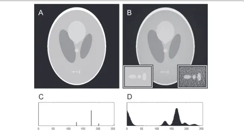
Taking a projection every 2 ° over a full 180 ° tilt range (and therefore with no missing wedge) and reconstructing the full image using a weighted backprojection algorithm with a ramp filter results in immediate changes. In particular, the intensity peaks in the histogram now overlap— meaning that there is now ambiguity in identifying

individual pixels based purely on their intensity. Figure 1 shows the original and reconstructed images, along with their histograms.

Thresholding

As Fig. 1 shows, even a perfect set of initial conditions (no noise, no missing wedge, perfect alignment of the projec-tions) introduces ambiguity into the reconstruction. The simplest way of obtaining a “discrete” image consisting of a small number of image intensities, each correspond-ing to a different type of material (see the histogram in Fig. 1c) from one with a continuously varying inten-sity, is to threshold the reconstruction—defining all pixels within a given intensity range as belonging to one class of material. Thresholding levels can be chosen manually by adjusting a control until the thresholded image looks cor-rect, or they can be determined using an algorithm such as the Otsu method [21].

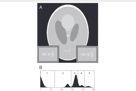
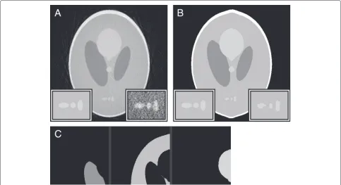
Figure 2 shows the effect of running a 5-level Otsu threshold operation [20] on the reconstruction in Fig. 1. Although the general shape of all the objects is retained, there are some very obvious mis-classifications in the form of a “speckle”. While it may be possible to improve the quality of the thresholded image by manually adjust-ing the threshold levels, this may be impractical in the case of large data sets and will not be of use when there is any overlap in image intensities between pixel classes.

Several methods exist for denoising an image or vol-ume, from simple Gaussian blurring (which will remove fine detail) to more advanced edge-preserving algorithms such as bilateral filtering. A recent review [23] showed that non-linear anisotropic diffusion (NAD) [24] is an effec-tive method for noisy reconstructions of biological mate-rial. Because the “speckle” already causes problems when analysing even a “perfect” reconstruction, we will use NAD filtering for all of the artefacted phantom images.

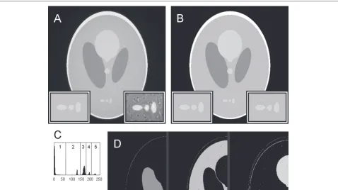
Figure 3 illustrates the effect of NAD on the “pure” reconstruction (perfect alignment, no noise, full angular range) from Fig. 1. The image is noticeably smoother after processing, which carries over to the thresholded image and can be seen in the image histogram. Comparing the inset regions in Fig. 3b) against Fig. 2a), there is noticeably less “speckle” in the NAD-filtered thresholded image.

(4)

Fig. 1Reconstruction artefacts raw (a) and WBP-reconstructed versions of a modified Shepp-Logan phantom (b) with their histograms shown in (c) and (d), respectively.Inset regionsin (b) are_×2 magnified portions of the lower central part—leftis from the source phantom,rightis from the reconstruction. Absolute intensity values should not be directly compared, as the reconstruction algorithm automatically scales the output data to saturate a 0—255 range. The contrast in theright insetof (b) has been enhanced for the purpose of improved visibility

small amount of “speckle” in the thresholded image, so the final result cannot be used for quantitative analysis without further processing.

Noise in the projections and projection misalignment

Figure 2 demonstrates that there are already several instances of mis-classification present even on “perfect” data. Real data will contain other sources of error—the simplest of which being shot noise, an inevitable conse-quence of quantum mechanics which is more prominent in low-current situations (the signal to noise ratio scales with√I, where I is the beam current). We simulate this by applying the RandomJ Poisson noise tool (built-in to Fiji) in additive mode with a mean of 0.5 to the sinogram (a composite image of all the projections) generated by the Radon transform tool, then reconstructing the image from the noised output.

Furthermore, if the projections are not perfectly aligned with respect to each other, additional errors will occur upon reconstruction. Alignment procedures usually con-sist of cross-correlation routines between subsequent images in the tilt series—either across the whole image or between manually indicated regions of the image (for instance, a low concentration of gold nanoparticles are sometimes added to samples before imaging to serve as fiducial markers). Alignment is usually more accurate

when carried out using fiducial markers because of their high contrast, but they can obscure parts of the sample through shadowing effects.

To show the effect of projection misalignment, we use an ImageJ macro to shift each projection by a random dis-tance with flat probability distribution between −1 and

+1 pixels along its length, using bicubic interpolation in the case of non-integer shifts. The misaligned data is then reconstructed as per the previous example.

(5)

Fig. 2Thresholded reconstruction.aThe result of a 5-level Otsu threshold on the reconstructed image in Fig. 1, and (b) the position of the threshold levels in the image histogram. Inset regions are×2 magnified from the phantom (left) and thresholded reconstruction (right)

Missing wedge

The other reconstruction issue we present is that of the missing wedge. As mentioned earlier, this is caused by reconstructing from a limited angular range (the maxi-mum possible is 180 °) and occurs for several reasons—the sample holder may obstruct the field of view at high tilt angles; the microscope’s goniometer may not be able to tilt through the full−90 °–+90 ° range, or the sample is in the form of a plane (as opposed to an isolated particle or a fabricated cylindrical pillar [26]) and images taken at high tilt angles have too high an effective sample thickness for good quality imaging. Unless tilt series are taken of pillar samples or individual particles and using a sample holder which allows full rotation without obstructions, there will always be a missing wedge of information for which to account.

To demonstrate the effect of the missing wedge, we use an angular range of −76 °–+76 ° (and therefore a missing wedge of 28 °), which corresponds approximately to the maximum usable angular range for most tomo-graphic experiments (unless free-standing needle samples are used).

(6)

Fig. 3Plain reconstruction, processed with NAD.aThe reconstruction from Fig. 1 but processed with NAD.bThe result of a 5-level Otsu threshold operation on the processed image.cThe histogram for (b) with the threshold levels indicated.dThe middle three threshold levels from thetop-left part of (a) displayed in separate images. Inset regions are×2 magnified from the phantom (left) and NAD-filtered reconstruction (right). The contrast in the right inset of (a) has been enhanced for the purpose of improved visibility

Application to real data

Finally, we apply these methods to a piece of real data acquired through electron tomography. The sample used here is a composite of silica nanoparticle aggregates inside a rubber matrix, the bulk sample being 25 % silica by vol-ume (investigated previously [7] by the authors using the technique demonstrated in this work).

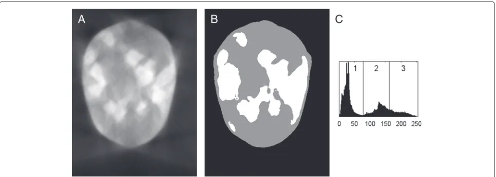
Figure 6 shows one slice from the experimental data. The missing wedge is visible in the form of fanning arte-facts at the top and bottom of the pillar, but the interior of the object does not appear to suffer from them as much as the WBP reconstruction in Fig. 5. The use of SIRT in this reconstruction as opposed to the WBP used for the pre-vious examples may have had a small positive impact on reconstruction quality.

The most important factor in analysing this experimen-tal data is that there is a large overlap between pixel intensities for the different classes—just as in the noised, misaligned reconstruction (Fig. 4), the histogram has no obvious delineation between the rubber- and silica-pixel intensity levels. The net result is that what would ordi-narily be separate silica particles have merged together in the thresholded image and that those which have not merged are larger than a cursory visual inspection of the unprocessed image would indicate.

As Fig. 7 shows, while applying NAD (using the same settings as for Fig. 3a) to the experimental data does make the image visually cleaner, it does very little about improv-ing the thresholded image. Whether due to sources of error (such as the missing wedge, noisy projections or other issues) or an innate inhomogeneity in the sample, the histogram still does not have three discrete peaks, parts of the image are still classified incorrectly (for instance, the left-most particles), and the thresholded image is still not usable for quantitative analysis.

There is another disadvantage to using post-processing techniques. Applying any kind of filter to an image will obviously alter it—and the output image may not neces-sarily have important features (such as edges) in the same place as the original image. While a good filter should not move objects around, the possibility remains, and as such, quantitative distance measurements may not be accurate on any images which have been post-processed.

An introduction to machine learning

(7)

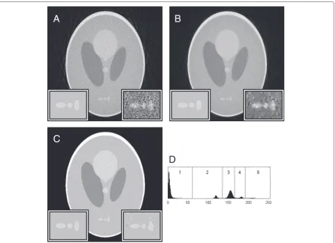
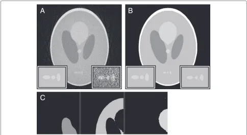
Fig. 4Noisy misaligned reconstruction, processed with NAD.aA WBP reconstruction of projections which have been randomly misaligned and given Poisson noise.bThe reconstruction from (a) processed with NAD.cThe result of a 5-level Otsu threshold operation on the processed image. dThe histogram for (b) with the threshold levels indicated.aInset regionsare×2 magnified from the phantom (left) and the plain reconstruction; bthe NAD-filtered reconstruction (right). The contrast in the right inset of (b) has been enhanced for the purpose of improved visibility

reconstructions remains a widespread technique. How-ever, there are two main downsides to manual segmenta-tion. Firstly is that since the operator has to go through each individual slice and manually draw every particle boundary, it is an extremely time-consuming technique. Secondly is that carrying out the same “procedure” twice will not give the exact same result—while an expert oper-ator will achieve very similar results if analysing the same reconstruction twice, the results will not be identical, nor will they be identical to the result of another oper-ator segmenting the same data. This is an unavoidable consequence of relying on human input.

The biggest drawback of manual segmentation is arguably the time requirement. The field of machine learning offers a solution to this—by “training” a com-puter to recognise parts of an image in the same way a human does, the computer should be able to classify a noisy image unattended, potentially faster than a human operator (dependent on the computer’s processing power

and memory) and presenting the same output when exe-cuted repeatedly on the same input. Machine learning is a deep, complicated field, and as such, we will not be describing it in depth here—the book by Witten and Frank [27] should serve as a good starting point for interested readers.

(8)

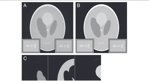
Fig. 5Missing wedge reconstruction, processed with NAD.aA WBP reconstruction of aligned, noiseless projections with a 28 ° missing wedge. bThe reconstruction from (a) but processed with NAD.cThe result of a manual threshold operation on the processed image.dThe histogram for (a) with the threshold levels indicated.aInset regionsare×2 magnified from the phantom (left) and the plain reconstruction;bthe NAD-filtered reconstruction (right). The contrast in the right insets of (a) and (b) has been enhanced for the purpose of improved visibility

(9)

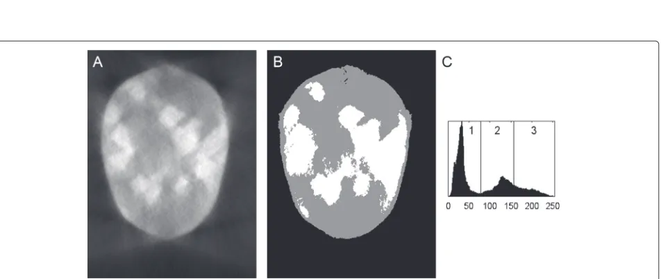
Fig. 7NAD-filtered experimental data.aA NAD-filtered version of Fig. 6a.bThe result of a 3-level Otsu threshold operation on the filtered reconstruction.cThe histogram for (a) with the threshold levels indicated

copies in those regions are then used as training data for a classifier algorithm. By default, Trainable Weka Segmen-tation uses a random forest algorithm [30], but another may be chosen if the operator desires.

When at least one region has been marked out for each class, the classifier algorithm is then run on the initial training data, and a sample output generated. The user is then able to look over the data and if a part of the image has been incorrectly classified, it can be marked with the correct class (not all of the incorrect areas need to be marked) and the classifier algorithm run again once the necessary corrections have been made. This process can be repeated as many times as necessary until the user is happy with the classification output.

This aspect is what sets machine learning aside from traditional processing steps. While it is not easy to obtain an exact definition of “machine learning”, it is related to the field of data mining, defined by Witten and Frank as “the process of discovering patterns in data which must be automatic or (more usually) semiautomatic. The pat-terns discovered must be meaningful in that they lead to some advantage” [27]. They also provide a definition of learning as follows: “Things learn when they change their behaviour in a way that makes them perform better in the future”. Because the software is not being told exact rules for image classification but is instead given examples and left to “figure out” the result on its own, and because this will usually result in a more accurate classification when applied to the data, it has effectively learned from the user input.

Note that since the output is strongly dependent on the training data, it will therefore still depend on the person doing the training—thus retaining one of the draw-backs of manual segmentation. Additionally, depending on the “complexity” of the data (such as when there is a

lot of pixel intensity overlap or other sources of uncer-tainty), training may take a long time—though never as long as performing a full manual segmentation. How-ever, the training data can be saved and applied to other images (assuming that they are similar enough), and the final classification step can run unattended, mitigating the manual segmentation drawbacks of non-repeatability and time consumption.

Using the Trainable Weka Segmentation software on tomographic reconstructions

Although the procedure is described above in the Meth-ods section, the image setup and the choice of options will have a significant effect on the quality of the final result. We therefore explain some of the workflow in more detail here to justify our choices.

(10)

The second step is to ensure that the training volume will fit inside RAM. If a large number of features are taken, the amount of RAM used can be significantly greater than the file size. To work around this, a substack consisting of every nth slice is taken from the reconstruction and training is carried out on that substack. This can be done using Fiji with the Make Substack command. For refer-ence, our reconstructions are usually on the order of 400

×400×850 voxels, and we take a substack consisting of every 15th slice (9.1 million voxels in total), which con-sumes approximately 10 GB of RAM during the training procedure.

The trimmed substack can now be used as training data, but before proceeding, the operator needs to define the number of classes within the image (for instance, vacuum, matrix and nanoparticle) and to select which training fea-tures will be used to classify the image. Because each image is different and because parts of an image will be recognised by different means (for instance, the difference between a small nanoparticle and an extended cell mem-brane), there is no universal set of training features which will classify every image. The operator must therefore have a basic understanding of what each training feature “sees” and whether or not it applies to their data.

As mentioned earlier, the ideal set of training features is dependent on which sources of contrast the image presents—both desired contrast in the form of desirable image features and errant contrast which the operator wishes to explicitly reject (such as missing wedge arte-facts). Because of this, we provide a short explanation for why individual features were chosen to use on our data—note that since it is possible that future versions of Trainable Weka Segmentation may offer a different fea-ture set, or change the way in which feafea-tures operate, it is advisable to check the software’s website [18] for a more up to date and in-depth description of exactly what each feature is calculating. In general, the training features can be grouped together as “seeing” different categories of image contrast such as: voxel intensity-averaging features (Gaussian blur, mean, minimum, maximum, median), edge-preserving intensity-averaging features (anisotropic diffusion, bilateral, Kuwahara), edge detection features (Sobel filter, derivatives), orientation features (Hessian, Gabor, structure), smoothly varying background subtrac-tion (Lipschitz), line detecsubtrac-tion (membrane projecsubtrac-tions), “blob” detection (difference of Gaussians, Laplacian), and non-directional local changes or noise (entropy, variance, neighbours)—all in addition to the raw source image (or the hue, saturation and brightness images in the case of a colour source).

Our choice of training features was as follows: Gaus-sian blur, median (voxel intensity averaging); anisotropic diffusion, bilateral, Kuwahara (edge-preserving averag-ing functions); Sobel filter, derivatives (edge detection);

Hessian, Gabor, structure (orientation detection); mem-brane projections (extended object detection); difference of Gaussians, Laplacian (object size detection); variance, entropy, neighbours (local noise level). We did not use the mean, minimum, maximum (voxel intensity) or Lipschitz (smoothly varying background subtraction) filters.

The first five filters, Gaussian blur, median, anisotropic diffusion, bilateral and Kuwahara, are all essentially aver-aging techniques which output something closely related to the source image but smoothed to reduce noise in some way. Since raw pixel intensity is the main way by which phases in both the phantom and the data are identified, a source of input from the intensity is required to form a complete analysis. Since all five of these filters produce a similar type of training feature, it should technically be workable to use only a subset of them (for instance, by eliminating the less sophisticated Gaussian blur) and still obtain a similar result, but we chose to use them all because without a time-consuming inspection of every data set with every filter type before processing, it is not obvious which filters show “better” detail.

The Sobel and derivative filters both detect changes in image intensity in a non-directional manner—edge detec-tion. This is required to locate the boundaries between phases.

Hessian, Gabor and structure filters detect the orienta-tion of image features—one very specific usage case for these is when compensating for missing wedge artefacts. If there is streaking or elongation in a particular direc-tion, the software will be able to recognise it using these filters and reject errant contrast—preventing something from being wrongly identified if only looking at the image intensity. Membrane projections operate in a similar man-ner, but measures extended linear objects and the angle at which they appear. This is particularly relevant to missing wedge “fanning” (which occurs at very specific angles), but may also be useful in differentiating a straight-edged crys-talline structure from a round amorphous structure of the same material.

Difference of Gaussian and Laplacian training features are “blob” detection filters, which measure the size of rel-atively small objects. This is useful not only for classifying objects based on their size (for instance, crystal or cell growth stages), but also for rejecting errant bright or dark spots in the image which are too small to be physical, but which would still trigger the intensity or edge detection features.

(11)

streaking from a missing wedge due to the blurring (and hence lower local variance due to smooth changes) that results, and possibly compensating for beam occlusion or detector efficiency changes by identifying a signal-to-noise level for each particular phase, separate from its raw pixel intensity.

It should be noted that the software will examine mul-tiple features simultaneously when performing the final classification. For instance, a combination of minor elon-gation in one direction with one particular intensity level might indicate the internal membranes of a mitochon-drion, while extended elongation in another direction (Hessian, Gabor or structure with membrane projections, at 26 degrees to the horizontal in our case) with another intensity level and a relatively low difference between intensity levels due to blurring (variance, entropy, neigh-bours) is characteristic of a missing wedge fanning arte-fact.

Machine learning and simulations

The “plain” reconstruction will serve as our first example. Compared to the Otsu-thresholded unprocessed image (Fig. 2a), the Trainable Weka Segmentation-processed image (Fig. 8) is significantly less noisy—in fact, it is almost indistinguishable from the source phantom (Fig. 1). The thresholded NAD-processed reconstruction in Fig. 3 was significantly cleaner than the unprocessed

reconstruction but still exhibited “speckle” which is not present in the Weka-processed reconstruction or the phantom. The “halo” effect seen at the edges of the NAD reconstruction (see Fig. 3d) is present to a smaller degree here, but it can be eliminated either through further train-ing of the classifier or, since the “halo” in this example is not a continuous line, possibly by removing all objects smaller than a certain size.

Training the classifier on this image took approximately 5 min—while this is a very long time compared to the few seconds required for a filter followed by a simple thresh-olding operation, the improvement in the accuracy of the final image is significant.

A more useful comparison would be with the noisy mis-aligned reconstruction, which is a better representation of the issues encountered with experimental data. Just as for the plain reconstruction, Fig. 9 is completely free of the “speckle” found in the NAD-processed thresholded image (Fig. 4). Despite the additional sources of error, the final image is still very similar to the source phantom, the only effect being that some edges on the various components inside the phantom appear “ragged” (for instance, see the three ellipses in the inset box). The “halo” on the outside of the phantom (Fig. 9c) in this case is smaller than the one from the “pure” reconstruction, most likely a side effect of the increased amount of training required to compensate for the poorer quality source image. This image required

(12)

Fig. 9Noisy misaligned reconstruction processed with Weka.aThe noisy misaligned reconstruction from Fig. 4.bThe same reconstruction but processed with Trainable Weka Segmentation.cThe middle three threshold levels from thetop-left partof (a) displayed in separate images.Inset regionsare_×2 magnified from the phantom (left) and reconstruction (right). The contrast in theright insetof (a) has been enhanced for the purpose of improved visibility

approximately 10–15 min to train the classifier—again, significantly more than the time required for a filter and threshold operation, but the result is far superior, and the classifier data will be useful for subsequent images in the stack (assuming that a full volume is being examined).

Properly trained machine learning software is also capa-ble of handling missing wedge fan artefacts much more effectively than an ordinary threshold or NAD filter, as can be seen in Fig. 10. The output is not perfect—the inset ellipses, for instance, are visibly distorted when compared to the phantom, but are significantly better than the result of the NAD filter+thresholding operation (Fig. 5). The other effect of a missing wedge, elongation in the direc-tion of the missing data, remains in the processed image (see the top and bottom of the object). While an expe-rienced operator may “know” that the image should be shorter than it appears, this information is not present within the reconstructed image and therefore neither the software nor the operator will be able to say exactly what the “real” geometry of the sample is. This is in contrast to noise or fan artefacts, where information on object boundaries is still present within the image, and the oper-ator or a trained classifier will be able to exactly mark the “correct” location of a boundary. Pure image-processing techniques such as NAD filtering or machine learning classification will not be able to compensate for missing

wedge elongation—this is an issue which would be more effectively solved by the reconstruction algorithm.

Machine learning and experimental data

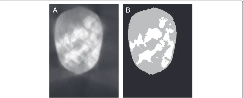
Our final example is that of the experimental data, which exhibits both noise and missing wedge artefacts (it is not possible to know a priori whether there was any mis-alignment in the projections). As Figs. 6 and 7 showed, global thresholding failed both with and without a non-linear anisotropic diffusion-filtering step beforehand. The machine learning approach (Fig. 11), on the other hand, achieved a very accurate classification of the image. While it is obviously impossible to judge exactly how accurate the result is without a “pure” source image to compare against, it visually achieves a very close match to what the human eye would mark out as the object boundaries.

(13)

Fig. 10Missing wedge reconstruction processed with Weka.aThe perfectly aligned, noiseless 28 ° missing wedge reconstruction from Fig. 5.bThe same reconstruction but processed with Trainable Weka Segmentation.cThe middle three threshold levels from thetop-left partof (a) displayed in separate images.Inset regionsare_×2 magnified from the phantom (left) and reconstruction (right). The contrast in the right inset of (a) has been enhanced for the purpose of improved visibility

Figure 12 shows the result of using the classifier on another slice from the same data set without any further training. There are some obvious mistakes (for instance, the top-right corner of the image), but these would be easily correctable with further training on more of the volume—this image is intended to show how a classifier

behaves when presented with similar data to that which it has been trained on.

The time required to train a classifier on a full substack will be significantly longer, as the software will need to re-classify each slice every time the input data is changed. It is also dependent on the quality of the input data—the

(14)

Fig. 12Weka-processed experimental data 2.aA different slice from the same data volume as Fig. 11., and the result of applying the classifier to that slice without further training (b)

classifier will be able to learn from “clean” images much more quickly and effectively than noisy, blurry images. We usually spend approximately 8–10 h training the classi-fier on volumes like the experimental data shown here to achieve a result with a similar accuracy to Fig. 11.

To re-state an earlier point, while more advanced recon-struction algorithms do exist which can minimise or completely eliminate artefacts such as these and reduce the need for post-processing, they are not the focus of this work. We accept that a reconstruction will not be perfect—containing reconstruction artefacts or actual inhomogeneities in the material and instead seek ways to obtain the most accurate final result despite starting from an imperfect image.

Comparison to other advanced post-processing techniques

It should be stressed that the work here is on the topic of image classification, not image segmentation. We define classification as where a “wide-spectrum” greyscale image is converted into a “discrete” greyscale image with a small number of grey levels, each grey level corresponding to one particular class of feature in the image (for instance, vacuum, silica and rubber for our experimental sample; or outer membrane, mitochondrion, cytoplasm and endo-plasmic reticulum for a biological cell). When applying such a procedure to projection and reconstruction from a simulated phantom, a perfect classification will pro-duce the source phantom as its output. Segmentation, on the other hand, is the breakdown of an image into discrete objects, or segments. Segmentation will produce geometrical information on each of these separate objects (for instance, their edges and centres) as its output. The two techniques are very closely related, and classifica-tion (for instance, by thresholding) is a useful first step

in segmentation, though some algorithms such as the watershed transform [31] can function on non-binarised data.

The purpose of the Trainable Weka Segmentation pro-cessing demonstrated here is to serve as a post-propro-cessing stage to improve the accuracy of further numerical analysis—by creating a cleaner “source” image to work from, a procedure such as the watershed transform will be able to create more accurate surface models from objects in the reconstruction, leading to an improvement in measured quantities such as particle size and spacing distributions.

Conclusions

We have demonstrated a machine learning method of processing imperfect tomographic reconstructions which provides for a much more accurate image classifica-tion than convenclassifica-tional thresholding and which does not require altering the source data with image filters before processing. The time required to train and process a reconstruction using the machine learning software is sig-nificantly longer than a simple filter and threshold oper-ation, but is likewise faster and more repeatable than a manual image classification and with comparable accu-racy. Finally, the software used for this processing is freely available in both binary and source form on multiple plat-forms, meaning that there are few practical barriers to its usage.

Competing interests

The authors declare that they have no competing interests.

Authors’ contributions

(15)

Acknowledgements

The research leading to these results has received funding from the European Research Council under the European Union’s Seventh Framework Programme (FP7/2007-2013)/ERC grant agreement 291522-3DIMAGE. The rubber-silica composite sample was provided by Michelin.

Received: 9 March 2015 Accepted: 21 June 2015

References

1. Crowther, RA, DeRosier, DJ, Klug, A: The reconstruction of a three-dimensional structure from projections and its application to electron microscopy. Proc. R. Soc. A.317(1530), 319–340 (1970). doi:10.1098/rspa.1970.0119

2. Gilbert, P: Iterative methods for the three-dimensional reconstruction of an object from projections. J. Theor. Biol.36(1), 105–117 (1972). doi:10.1016/0022-5193(72)90180-4

3. Midgley, PA, Ward, EPW, Hungria, AB, Thomas, JM: Nanotomography in the chemical, biological and materials sciences. Chem. Soc. Rev.36, 1477–1494 (2007). doi:10.1039/B701569K

4. Banhart, J (Ed): Advanced Tomographic Methods in Materials Research and Engineering. Oxford University Press, Oxford, UK (2008). ISBN: 9780199213245

5. Midgley, PA, Weyland, M: 3D electron microscopy in the physical sciences: the development of z-contrast and EFTEM tomography. Ultramicroscopy.

96(3–4), 413–431 (2003). doi:10.1016/S0304-3991(03)00105-0 6. Ikeda, Y, Katoh, A, Shimanuki, J, Kohjiya, S: Nano-structural observation of

in situ silica in natural rubber matrix by three dimensional transmission electron microscopy. Macromol. Rapid Commun.25(12), 1186–1190 (2004). doi:10.1002/marc.200400053

7. Staniewicz, L, Vaudey, T, Degrandcourt, C, Couty, M, Gaboriaud, F, Midgley, P: Electron tomography provides a direct link between the payne effect and the inter-particle spacing of rubber composites. Sci. Rep.

4(2014). doi:10.1038/srep07389

8. Zeˇcevi´c, J, van der Eerden, AMJ, Friedrich, H, de Jongh, PE, de Jong, KP: Heterogeneities of the nanostructure of platinum/zeolite Y catalysts revealed by electron tomography. ACS Nano.7(4), 3698–3705 (2013). doi:10.1021/nn400707p

9. Yates, TJV, Thomas, JM, Fernandez, J-J, Terasaki, O, Ryoo, R, Midgley, PA: Three-dimensional real-space crystallography of mcm-48 mesoporous silica revealed by scanning transmission electron tomography. Chem. Phys. Lett.418(4–6), 540–543 (2006). doi:10.1016/j.cplett.2005.11.031 10. Arslan, I, Walmsley, JC, Rytter, E, Bergene, E, Midgley, PA: Toward

three-dimensional nanoengineering of heterogeneous catalysts. J. Am. Chem. Soc.130(17), 5716–5719 (2008). doi:10.1021/ja710299h 11. Gilbert, PFC: The reconstruction of a three-dimensional structure from

projections and its application to electron microscopy. ii. direct methods. Proc. R. Soc. B.182(1066), 89–102 (1972). doi:10.1098/rspb.1972.0068 12. Batenburg, KJ, Bals, S, Sijbers, J, Kübel, C, Midgley, PA, Hernandez, JC,

Kaiser, U, Encina, ER, Coronado, EA, Tendeloo, GV: 3d imaging of nanomaterials by discrete tomography. Ultramicroscopy.109(6), 730–740 (2009). doi:10.1016/j.ultramic.2009.01.009

13. Goris, B, den Broek, WV, Batenburg, KJ, Mezerji, HH, Bals, S: Electron tomography based on a total variation minimization reconstruction technique. Ultramicroscopy.113, 120–130 (2012).

doi:10.1016/j.ultramic.2011.11.004

14. Leary, R, Saghi, Z, Midgley, PA, Holland, DJ: Compressed sensing electron tomography. Ultramicroscopy.131, 70–91 (2013).

doi:10.1016/j.ultramic.2013.03.019

15. Shepp, LA, Logan, BF: The fourier reconstruction of a head section. IEEE Trans. Nucl. Sci.21(3), 21–43 (1974). doi:10.1109/TNS.1974.6499235 16. Thévenaz, P: An ImageJ Plugin for the Creation of the Shepp-Logan

Phantom. http://bigwww.epfl.ch/thevenaz/shepplogan/

17. Farrell, D: Radon Transform Plugin for ImageJ. http://imagej.net/plugins/ radon-transform.html

18. Schindelin, J, Arganda-Carreras, I, Frise, E, Kaynig, V, Longair, M, Pietzsch, T, Preibisch, S, Rueden, C, Saalfeld, S, Schmid, B, Tinevez, J-Y, White, DJ, Hartenstein, V, Eliceiri, K, Tomancak, P, Cardona, A: Fiji: an open-source platform for biological-image analysis. Nat Meth.9(7), 676–682 (2012) 19. Tosa, Y: Multi Otsu Threshold Plugin for ImageJ. http://imagej.net/

plugins/multi-otsu-threshold.html

20. Liao, P, Chew, T, Chung, P: A fast algorithm for multilevel thresholding. J. Inf. Sci. Eng.17(5), 713–727 (2001)

21. Otsu, N: Threshold selection method from gray-level histograms. IEEE Trans. Syst. Man, Cybern.9(1), 62–66 (1979)

22. Fernández, J-J, Li, S: An improved algorithm for anisotropic nonlinear diffusion for denoising cryo-tomograms. J. Struct. Biol.144(1-2), 152–161 (2003). doi:10.1016/j.jsb.2003.09.010

23. Narasimha, R, Aganj, I, Bennett, AE, Borgnia, MJ, Zabransky, D, Sapiro, G, McLaughlin, SW, Milne, JLS, Subramaniam, S: Evaluation of denoising algorithms for biological electron tomography. J. Struct. Biol.164(1), 7–17 (2008). doi:10.1016/j.jsb.2008.04.006

24. Frangakis, AS, Hegerl, R: Noise reduction in electron tomographic reconstructions using nonlinear anisotropic diffusion. J. Struct. Biol.

135(3), 239–250 (2001). doi:10.1006/jsbi.2001.4406

25. Batenburg, KJ, Sijbers, J: Optimal threshold selection for tomogram segmentation by projection distance minimization. IEEE Trans. Med. Imaging.28(5), 676–686 (2009). doi:10.1109/TMI.2008.2010437 26. Kawase, N, Kato, M, Nishioka, H, Jinnai, H: Transmission electron microtomography without the “missing wedge” for quantitative structural analysis. Ultramicroscopy.107(1), 8–15 (2007). doi:10.1016/j.ultramic.2006.04.007

27. Witten, IH, Frank, E: Data Mining: Practical Machine Learning Tools and Techniques. 2nd edn. Morgan Kaufman, Burlington, Massachusetts, US (2005)

28. Hall, M, Frank, E, Holmes, G, Pfahringer, B, Reutemann, P, Witten, IH: The WEKA Data Mining Software: An Update. SIGKDD Explor.11(1), 10–18 (2009)

29. Sommer, C, Straehle, C, Koethe, U, Hamprecht, FA: Ilastik: Interactive learning and segmentation toolkit. In: Biomedical Imaging: From Nano to Macro, 2011, p. 230,233. IEEE International Symposium on, (2011). doi: 10.1109/ISBI.2011.5872394

30. Breiman, L: Random forests. Mach. Learn.45(1), 5–32 (2001). doi:10.1023/A:1010933404324

31. Meyer, F: Topographic distance and watershed lines. Signal Process.

38(1), 113–125 (1994). doi:10.1016/0165-1684(94)90060-4