Fundus Image Classification Using Two Dimensional Linear Discriminant Analysis and Support Vector Machine

(1)

Infogain Publication (Infogainpublication.com) ISSN : 2454-1311

Fundus Image Classification Using Two

Dimensional Linear Discriminant Analysis and

Support Vector Machine

Wahyudi Setiawan, Fitri Damayanti

Department of Information System, Trunojoyo University, Bangkalan, East Java, Indonesia

Abstract— It is constructed in this study a classification

system of diabetic retinopathy fundus image. The system consists of two phases: training and testing. Each stage consists of preprocessing, segmentation, feature extraction and classification. The tested image comes from the MESSIDOR dataset which has a total of 100 images. The number of classes to be classified consists of four classes with each class consists of 25 images. The classes are normal, mild, moderate and severe of Diabetic retinopathy. In this study, the level of preprocessing uses grayscales green channel, Wavelet Haar, Gaussian filter and Contrast Limited Adaptive Histogram Equalization. The level of segmentation uses masking as a process of doing the subtracting operation of between the original image and the masking image. The purpose of the masking is to split between the object and the background. The feature extraction uses Two Dimensional Linear Discriminant Analysis (2DLDA). The classification uses Support Vector Machine (SVM). The test results of some scenarios show that the highest percentage of accuration of the system is up to 90%.

Keywords— Diabetic Retinopathy, Two Dimensional Linear Discriminant Analysis, Support Vector Machine, Fundus Image, MESSIDOR.

I. INTRODUCTION

Diabetic Retinopathy (DR) is a disease of the eye as a result of complications of Diabetes Mellitus (DM). The Symptom of DR is a decrease in vision sharpness; moreover, it is a blindness. The percentage of patients with diabetes mellitus who suffered DR is quite high reaching around 40% to 50%. Normally, the symptom of DR only comes with patients who have been over than 10 years of experiencing DM. DR has been often easily detected for the patient with old age that the patient is unaware of the DM [1]. DR can cause abnormalities in the retina. The abnormality has five categories, namely [2]:

a. Microaneurism is a bulging of capillary wall

especially in the area of veins shaped like a small red spot which is close to the veins.

b. Hemorrhages usually appear on the capillary wall

and are visible from the spot of blood out of the veins which are dark red and is larger than microaneurism.

c. Hard exudates are lipid infiltration into the retina

with yellowish and irregular shape.

Soft exudates or often called cotton wool patches are a retinal ischemia with yellow and white spots.

d. Neovascularization is a new blood vessel in the

tissue surface, irregularly shaped, winding and in groups.

The results of the medical diagnosis of fundus image show the level of DR disease being experienced. There are four classes of diagnostic results, namely: Class Normal, level 1 of DR, level 2 and of level 3 of DR. Here is the characteristic of the DR level obtained from the fundus image [2]:

a. Normal

No Microaneurysm AND No Hemorrhages

b. Mild Diabetic Retinopathy

Microaneurysm is between more than 0 to less than or equal to 5 AND No Hemorrhages

c. Moderate Diabetic Retinopathy

Microaneurism is between more than 5 to less than 15 OR Hemorrhages is between more than 0 to less than 5 AND No Neovascularization

d. Severe Diabetic Retinopathy

Microaneurysm is more than or equal to 15 OR Hemorrhages is more than 5 AND

Neovascularization is equal to 1

II. RELATED WORKS

(2)

International Journal of Advanced Engineering, Management and Science (IJAEMS) [Vol-2, Issue-10, Oct- 2016] Infogain Publication (Infogainpublication.com) ISSN : 2454-1311

Median Filter, Adaptive Histogram Equalization. It is then further processed on Boundary Tracing using edge detection, Adaptive Threshold & Centroid, Optic Disk Localization and Vessel Extraction. The next process is

by doing Image Segmentation, namely Class

Segmentation and Class Boundary. The results of the study [4] show 97.1% of sensitivity, specificity 98.3%. The following research is the automatic detection of diabetic retinopathy using feature extraction and classification of Support Vector Machine. This study discusses the feature extraction of Gray Level Co-occurrence Matrix (GLCM) and classification using Support Vector Machine method. The classification is divided into two classes, namely Normal and Diabetic Retinopathy. The imagery used is around 200. The research result shows that the system accuracy is reaching 93% [5]. In the study [6] use the same classification method which is an SVM. The difference lies in the preprocessing and the feature extraction used. In the study [6], the preprocessing being used are green channel, Contrast Limited Adaptive Histogram Equalization

(CLAHE), filtering, Contrast Enhancement,

Morphological Operation, Optic Disc Elimination. Statistical Feature is used for the Feature Extraction process. 92% of Sensitivity, 80% of Specificity, 90% of accuracy.

The further research is the detection of diabetic retinopathy using machine learning. The class is divided into two (2), namely Non-Proliferative Diabetic

Retinopathy (NPDR) and Proliferative Diabetic

Retinopathy (PDR). The methods used include

Probabilistic Neural Network (PNN), Bayesian

Classification and Support Vector Machine. The imagery used for training are 100 images, and 250 images of testing. The valid percentages are 89.6% for PNN, 94.4% for Bayesian, 97.6% for SVM [7].

In [8], CLAHE, median filtering and image catenation on four tiles are method for preprocessing. In the study [9], the preprocessing used are the green channel, CLAHE, mathematical morphology, optical disks detection and removal and max tree algorithms. Classification used SVM. The trial results show 96.9% of sensitivity, 100% of Specificity.

In [10] the preprocessing method used applies Green Channel, Filtering, Image Enhancement, morphological

Operation, Hard exudates Segmentation, feature

extraction. The classification uses Adaptive Neuro Fuzzy Inference System (ANFIS) and Extreme Learning Machine (ELM).

The research [11] is a review of methods for DR Classification. This research include preprocessing, feature extraction method such as optic disc, flovea vessel blood and abnormal feature extraction. It can classify 5

class i.e normal, Mild NPDR, Moderate, Severe and Proliferative Retinopathy.

Diagnosis of DR based on feature extraction is the next research. This research implementing Neuro Fuzzy for feature extraction[12]. In reference to [13], the research uses Fuzzy C Means segmentation. In the process of preprocessing, there is a change of pilot image to binary image which is then performed a labeling on the objects and the holes. The next process is the boundary detection and classification using FCM.In [14] , the research proposed system for detecting DR. The system consist of

preprocessing, morphological operation, feature

extraction and SVM Classifier.

The research [15] using several methods i.e preprocessing used compressed image 640x480 pixel using bi-cubic interpolation, detection of optic disc, blood vessels, white lesions, red lesions. The test produces 80% and 50% for sensitivity and spesificity.

In [16] , the research is used convolutional Neural Network for detecting DR. The next research focus is to [17] discuss the stages of retinopathy detection using preprocessing, feature extraction and classification. Preprocessing uses image enhancement, edge detection, morphological operations, thinning to only 1 pixel, scanning window analysis (SWA). Overal accuracy of proposed method is 92.72%

III. METHODOLOGY

This study consists of two parts: training and testing. Each section consists of four stages: preprocessing, segmentation, feature extraction and classification. The research methodology that was created is shown in Figure 1.

3.1 Preprocessing

Preprocessing aims to improve the quality of the image by manipulating the parameters of the image. In this study, the preprocessing process consists of the grayscale green channel, Gaussian filter, Contrast Limited Adaptive Histogram Equalization (CLAHE).

3.2 Segmentation

(3)

Infogain Publication (Infogainpublication.com

Fig.1 : Retinopathy Research Methodology

(a) (b)

Fig.2 : (a) before the image preprocessing, (b) the image masking, (c) the image as a result of masking

3.3 Feature Extraction

Feature extraction is a retrieval characteristic of an object image which is a unique value differentiator as to compare with another object. The feature extraction is applied to checking the Cartesian coordinates, namely horizontal, vertical, diagonal right and left diagonal.

3.3.1 Two-Dimensional Linear Discriminant Analysis (2DLDA)

2DLDA is the enhanced method of LDA. Firstly LDA 2D matrix is transformed into the form of a one

vector image, whereas in 2DLDA or it is called a direct image projection technique, the matrix 2D image does not need to be transformed into the form of vector image but its image matrix distribution can be formed directly by using the original image matrix.

{A1,….,An} is the n image matrix, whereas

the r x c image. Mi (i=1,…,k) is the average training

image of the class from the i and M which is the average

of all the training data.

l

₁ x

l

₂ is the dimensional space

of L

⊗

R, whereas

⊗

is to show the tensor product,

Infogainpublication.com)

Retinopathy Research Methodology

(c)

(a) before the image preprocessing, (b) the image masking, (c) the image as a result of masking

Feature extraction is a retrieval characteristic of an object image which is a unique value differentiator as to object. The feature extraction is applied to checking the Cartesian coordinates, namely horizontal, vertical, diagonal right and left diagonal.

Dimensional Linear Discriminant Analysis

2DLDA is the enhanced method of LDA. Firstly LDA 2D matrix is transformed into the form of a one-dimensional vector image, whereas in 2DLDA or it is called a direct image projection technique, the matrix 2D image does not need to be transformed into the form of vector image but can be formed directly by

image matrix, whereas Ai (i=1,…,k) is

) is the average training which is the average

is the dimensional space

is to show the tensor product, L

covers {u1,…,u

l

₁} and R covers {

is defined with two matrixes

[v1,..,v

l

₂] [18].

Feature extraction method is for finding the that the original image space

dimensional image space as

space is obtained by a linear transformation of the distance between classes in

class in Dw are defined as follows:

R M M L n Db k i i T

i ( )

1 − =

∑

= 2 F 2 1 ) ( F i k i x T R M X L Dw i − =

∑ ∑

= ∈Π

Whereas F is Frobenius norm

Reviewing that 2

F

A

= P

for matrix A and thus the equation of (3) and (4 represented more.

Db = trace ( ₍ ₎

1 RR M M L n k i i T i −

∑

=

Dw = trace ( ₍ ₎

1 RR M X L i k i x T i −

∑ ∑

= ∈Π

Similarly, LDA, 2DLDA method is to find the matrix and R, so that the class structure of the original space remains in the projection room, so the benchmark (criterion) can be defined as:

J1(L,R) = max W

b

D

.

It is clear that the equation (5) consists of a matrix transformation of L and R. Optimal transformation matrix of L and R can be obtained by maximizing

minimize Dw. However, it is very difficult to calcul

optimal of L and R simultaneously. Two optimization functions can be defined to obtain

R, L can be obtained by completing an optimization

function as follows:

J2(L) = max trace ((LTS R WL)

-Where:

S_bR = k T i

i

M

RR

n

(

)

(

1

−

∑

=

S_WR = ₍ ₎ ₍

1 T i k i x RR M X i −

∑ ∑

= ∈Π

Noting that the matrix size of

are smaller that the size of

S

For a defitnite L, R can be obtained by completing an optimization function as follows:

) ISSN : 2454-1311

covers {v1,..,v

l

₂}, and thus it

is defined with two matrixes L = [u1,…,u

l

₁] and R =

Feature extraction method is for finding the L and R, so

that the original image space - Ai is converted into

low-dimensional image space as Bi=LTAiR.. Low dimensional

space is obtained by a linear transformation of L and R,

the distance between classes in Db and the distance of

are defined as follows:

(1)

2

F

(2)

Frobenius norm.

trace (ATA) = trace (AAT) is

and thus the equation of (3) and (4) can be

) ) (M M TL

i

T ₋ (3)

). ) (X M L

RR T

i

T ₋ (4)

Similarly, LDA, 2DLDA method is to find the matrix L , so that the class structure of the original space remains in the projection room, so the benchmark (criterion) can be defined as:

. (5)

It is clear that the equation (5) consists of a matrix . Optimal transformation matrix

can be obtained by maximizing Db and

. However, it is very difficult to calculate the simultaneously. Two optimization functions can be defined to obtain L and R. For a definite can be obtained by completing an optimization

-1_(LT_SR

b L)) (6)

T

i

M

)

(

−

(7)

, )

(X−M_i T (8)

Noting that the matrix size of

S

_WR and SR_b are r x r which

R W

S

and S_bR in classical LDA.

(4)

J3(R) = max trace ((RTS L WR)

-1_(RT_SL

bR)), (9)

Where:

S_bL = ₍ ₎ ₍ ₎

1 M M LL M M n i T T k i i

i − −

∑

=

(10)

And,

S_WL = ₍ ₎ ₍ _).

1 i T T i k i x M X LL M X i − −

∑ ∑

= ∈Π (11)

3.4 Classification Using SVM

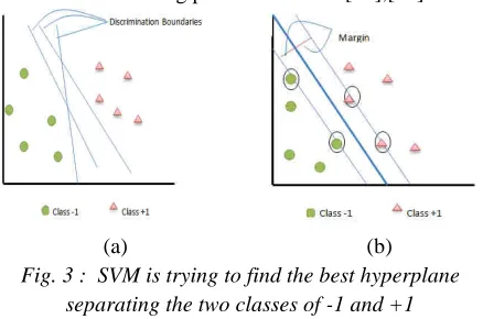
SVM concepts can be explained simply as an attempt to find the best hyperplane which serves as a separator of two classes in the input space. Hyperplane in a d-dimensional vector space is the affine subspace dimension of d-1 which divides the vector space into two parts where each corresponds to the different classes.

Figure 3 shows several patterns that are members of two classes: +1 and -1. Patterns belong to the class -1 is symbolized by the pink color (triangle), while the pattern on the class +1 is symbolized by the green color (circle). Problem of classification can be translated by figuring out a line (hyperplane) that separates between the two groups. Various alternatives of line separator (discrimination boundaries) are shown in Figure 3 (a).

Hyperplane as the best separator between the two classes can be found by measuring the margin of the hyperplane while looking for the maximum points. Margin is the distance between the hyperplane to the nearest pattern of each class. The closest pattern is called a support vector. The solid line in Figure 3 (b) shows the best hyperplane which is located right in the middle of the second grade while the red and yellow dots in black circle are the support vector. The attempts to locate this hyperplane are the core of the learning process on SVM [19],[20].

(a) (b)

Fig. 3 : SVM is trying to find the best hyperplane separating the two classes of -1 and +1

The data provided are denoted as

x

_i

∈

ℜ

d

r

, while for

each label is denoted with

y

_i

=

{

+

1 ,

−

1 }

for i = 1,2,3 ....

l Where l is the number of the data. It is assumed that the

second class of -1 and +1 can be separated completely by hyperplane with d dimension, which is defined as follows

0 =

+

⋅

x

b

w

r

(12)

w

r

pattern that includes class -1 (negative samples) can be

formulated as a pattern that satisfies inequality

1

− ≤ + ⋅x b

wr r (13)

While

w

r

pattern including the classes +1 (positive

samples) is

1 +

≥

+

⋅

x

b

w

r

(14)

To have the biggest margin is by maximizing the value of the distance between the hyperplane and the

closest point namely

w

r

1

. It can be formulated as a

Quadratic Programming (QP) problem, which is by

finding the minimum point of the equation that is finding the minimum point of the equation (15) with regard to constraint equation (16).

2

2 1 ) (

min w w w

r

r τ =

, (15)

(

x w b

)

i

y_i r_i⋅r+ −1≥0, ∀

(16) This problem can be solved with a variety of computational techniques, including Lagrange Multiplier.

(

)

∑

= − + ⋅ − = l i i i

i y x w b

w b w L 1 2 )) 1 ) ( ( 2 1 ,

, r r r

r

α

α (17)

with i = 1, 2, …, l .

αi are Lagrange multipliers, which is zero or positive

(αi≥0). The optimal value from equation (17) can be

calculated by minimizing the L and b, and maximize L to

αi. With regard to the nature that at the point of optimal

gradient L = 0, the equation (17) can be modified as the

maximization of problem that only contains αi, as the

below equation of (18).

, 2 1 1 , 1

∑

= = − l i i j i j i j i l i

i yy xx

r r

α

(18)

Where: 0 ) ,..., 2 , 1 ( 0 1 = = ≥

∑

= i l i i

i i l α y

α . (19)

From the result of this calculation αi is obtained with its

most positive value. Data were correlated with positive αi,

it is then so called as a support vector.

IV. RESULT

The testing scenario is achieved by using a dataset of Messidor test. The number of images used are 100 images consisting from 25 normal, 25 mild DR, 25 moderate DR , and 25 severe DR. In addition to that there are some uses of varying of data training, data test and projections dimensional variations of rows and columns. Moreover the conduct of varying the data training sequence is to gain the highest percentage.

(5)

Infogain Publication (Infogainpublication.com) ISSN : 2454-1311

been conducted some trials with 2DLDA + kNN method for comparison.

Table.1: The test results of kNN Classification ∑

training data

∑

testin g data

Acc.

40 20 68,33%

60 20 77,50%

80 20 80%

Table.2: The test results of SVM Classification ∑

training data

∑

testing data

Acc.

40 20 73,33%

60 20 80%

80 20 90%

The trial results show that the more the data trained, the better the accuracy. The percentage of accuracy with the more trained method of SVM is better with a 90% of maximum; compared with kNN method with its 80% of maximum.

V. CONCLUSION

There are two important variables that affect the success rate of introduction which are the sequence variations of training samples per class used and the number of training samples per class used. From the results of trials using kNN show the rate of optimal recognition accuracy is 80%, while the test results using methods SVM show the rate of optimal recognition accuracy is 90%

.

ACKNOWLEDGEMENT

The author would like to thank DRPM DIKTI (of Higher Education), which has funded this research in the form of competitive grants research budget, the year of 2016. This study is the 2nd year of the two years research plan.

REFERENCES

[1] M.Henricsson, L.Nystrom, G. Blohme,”The

Incidence of Retinopathy 10 years after Diagnosis in Young Adult People with Diabetes, DiabetesCare, Vol 26 No 2, February 2003

[2] M.Kuivalainen, Retinal Image Analysis using

Machine Vision, M.Sc Thesis, Lappreenranta University of Technology, Finland, 2005.

[3] A.Sopharak, B.Uyyanonvara, S.Barman and T.

Williamson,”Automatic Microaneurysm Detection from Non Dilated Diabetic Retinopathy Retinal Image, Proceedings of the world Congress on Engineering, Vol II, Londok. UK, July 2011

[4] A. Kumar, A.K Gaur and M. Srivastava, “A Segment

based Technique for Detecting Exudate from Retina Fundus Image, Procedia Technology, Vol 6, pp: 1-9, 2012

[5] D. Selvathi, N.B Prakash and N.

Balagopal,”Automated Detection of Diabetic

Retinopathy for Early Diagnosis using Feature Extraction and SVM, International Journal of Emerging Tachnology and Advanced Engineering, Vol 2 Issue 11, pp: 762-767, 2012

[6] C.Aravind, M.Ponnibala and S.Vijayachitra,

“Automatic Detection of Mycroaneurysms and Classification of Diabetic Retinopathy Images using SVM Technique, International Journal of Computer Applications, pp : 18 – 22, 2013

[7] R.Priya and P. Aruna,”Diagnosis of Diabetic

Retinopathy using Machine Learning

Techniique”,ICTACT Journal on Soft Computing, Vol 3 Issue 4, July, 2013

[8] N.S. Datta, H.S. Dutta, M.De, S.Mondal, “An

Effective Approach : Image Quality Enhancement for Microaneurysms Detection of Non Dilated Retinal Fundus Image, Procedia Technology Vol 10, pp: 731-737, 2013

[9] M.Faisal, D.Wahono, I.K.E. Purnama, M.Hariadi and

M.H Purnomo, “Classification of Diabetic

Retinopathy Patients using SVM based on Digital Retinal Images, Journal of Theoritical and Applied Information Technology, Vol 59 No 1, pp: 197-204, June 2014

[10]S. Vasanthi and R.S.D.W Banu, “Automatic

Segmentation and Classification of Hard Exudates to Detect Macular Edema in Fundus Images, Journal of Theoritical and Applied Information Technology, Vol 66 No 3, Aug 2014

[11]M.J.Paranjpe and M.N kakatkar,”Review of Methods

for Diabetic Retinopathy Detection and Severity Classification”, International Journal of Research in Engineering and Technology, Vol 3 Issue 3, pp: 619 – 624, March 2014

[12]K.Latha and S.G. Durga, “Diagnosis of Diabetic

Retinopathy Based on Feature Extraction”,

International Journal of Innovative Research in Science, Engineering and Technology, Vol 3 Spesial Issue 3, March 2014

[13]R.Samad, M.S.F. Nasarudin, M.Mustafa, D.Pebrianti,

M.R.H. Abdullah, “Boundary Segmentation and Detection of Diabetic Retinopathy in Fundus Image, Jurnal Teknologi, Vol 77 No 6, pp: 25-28, 2015

[14]R.S. Maher, S.N. Kayte, S.T. Meldhe and M.

Dhopeswarkar, “Automated Diagnosis Non

(6)

of Computer Applications, Vol 125 No 15, pp: 7 – 10, September 2015

[15]P.N.S. Kumar, R.U Depak, A. Sathar, V.

Sahasranamam, R.R. Kumar, “Automated Detection System for Diabetic Retinopathy using Two Field Fundus Photography”, Procedia Computer Science, 93, pp:486-494, 2016

[16]H.Pratt, F.Coenen,D.M.Broadbent, S.P. Harding and

Y. Zheng, “Convolutional Neural Networks for Diabetic Retinopathy”, Procedia Computer Science, 90, pp: 200 -205, 2016

[17]P.Panchal, R.Bhojani and T. Panchal, “An Algorithm

for Retinal Feature Extraction using Hybrid Approach”, Procedia Computer Science, 79, pp: : 61-68, 2016

[18]Z. Liang, , Y. Li , P. Shi, , “A note on

two-dimensional linear discriminant analysis”, Pattern

Recognition. 2122-2128. 2008.

[19]J.C. Burges , A Toturial on Support Vector Machines

for Pattern Recognition, Data Mining and Knowledge Discovery, 2(2):955-974. 1998.

[20]J.Weston, “Support Vector Machine and Statistical