Performance Analysis of Quantitative Attributes
Inverse Classification Problem
Aiguo Li
School of Computer Science and Technology, Xi’an University of Science and Technology, Xi’an, China Email: [email protected]
Xin Zhou and Jiulong Zhang
School of Computer Science and Technology, Xi’an University of Science and Technology, Xi’an, China Computer Science and Engineering, Xi’an University of Technology, Xi’an, China
Email: [email protected], [email protected]
Abstract
—
Most inverse classification algorithms address discrete attributes and can not deal with quantitative attributes. In order to overcome the disadvantage, the discretization algorithms are applied to the inverse classification algorithms, and the main idea is: firstly, a group of feature attributes are selected by using feature selection algorithm; then, the quantitative attributes are discretized by using discretization algorithms, and the inverted statistics are constructed on the training samples; finally, the test samples are analyzed in order to classify and estimate the missing values. Experimental results on IRIS and Ecoli datasets show that this method could find the class label effectively and estimate the missing values accurately. The performance of the equal-width histogram method is better in the inverse classification problem of quantitative attributes.Index Terms—Quantitative Attributes, Inverse Classification, Discretization algorithms
I. INTRODUCTION
The idea of inverse classification is that changes are made in the independent variables of a sample so that the sample can be classified into a more desirable class [1-3]. The inverse classification algorithm distinguishes itself from traditional classification algorithms with its inverse processing. The algorithm lays emphasis on analysis of the training samples and the test samples, with the class attributes completely defined. The values of attributes are adjusted till the desirable classification result is obtained.
The inverse classification algorithm was proposed by [3] which is a scalable and effective classification algorithm. In order to obtain the desirable classification result by adjusting the values of attributes, firstly, a group of key feature attributes are selected, then, the inverted statistics are constructed on the training data, finally, the test samples are analyzed in order to be classified and to estimate missing values. The training samples and test samples must be completely defined if they are used for classification; and features are incompletely defined and class attributes are completely defined in the test samples if they are used to estimate missing values. However, the training samples must have discrete values when the inverted statistics are constructed, and the test samples are discrete when the values of features are adjusted. To tackle this drawback, three methods are applied to convert the quantitative attributes into categorical form.
The performance of inverse classification on quantitative attributes is estimated, and the influences of discrete regions and discretization methods are analyzed.
II. DISCRETIZATION
The inverse classification algorithm assumes that all the attributes in the data set are discrete. The key of inverse classification on quantitative attributes is how to convert the quantitative attributes into categorical form. In this paper, three discrete algorithms namely, equal-width histogram (WH), equal-depth histogram (DH) and equal cumulative probability of Gaussian distribution (CGD) [4] are used to convert quantitative attributes into categorical form.
The main idea of RP is: assume that the dataset obeys the standard normal distribution, so the breakpoints split the Gaussian envelope into α equal-sized areas, and we can look up these breakpoints in a statistical table. For example, in Table 1, the values of α changes from 2 to 9, and the corresponding breakpoints β are listed below.
Once the breakpoints are obtained, the data sets could be discretized by the following methods. Assume that the datasetS containsN records of dimensionalityD. The process of discretization includes three steps:
Step 1: Normalization:
TABLEI.
THE BREAKPOINTS OF EQUAL CUMULATIVE PROBABILITY
β α
2 3 4 5 6 7 8 9
P1 0 -0.43 -0.67 -0.84 -0.97 -1.07 -1.15 -1.22
P2 0.43 0 -0.25 -0.43 -0.57 -0.67 0.76
P3 0.67 0.25 0 -0.18 -0.32 -0.43
P4 0.84 0.43 0.18 0 -0.14
P5 0.97 0.57 0.32 0.14
P6 1.07 0.67 0.43
P7 1.15 0.76
] [ ] [ ] [ ] ][ [ ] ][ [ j Min j Max j Min j i S j i S − −
=
(1)
wherei=1,2,3...N,j=1,2,3...D,S[i][j]denotes the j-th
attribute value of the i-th record,Max[j]denotes the
maximum value of the j-th dimension,Min[j]is the
minimum value of the j-th dimension.
Step 2: Standardization:
] [ ] [ ] ][ [ ] ][ [ j j E j i S j i S σ −
= (2)
wherei=1,2,3...N,j=1,2,3...D,S[i][j]denotes the j-th
attribute value of the i-th record,E[j]denotes the mean of
the j-th dimension,σ[j]is the standard deviation of the j-th dimension.
Step 3: Discretization: Define the number of discrete regionsK, finding theP1...Pk−1while α is equal to K
from Table 1. We define (−∞,P1]...(Pk−2,Pk−1],(Pk−1,+∞) as the K discrete regions. Finally, we can discretize the
data set by the K discrete regions.
III. INVERSE CLASSIFICATION PROBLEM AND ITS
APPLICATIONS
The main idea of the inverse algorithm is: firstly, select a group of features and perform the discretization algorithms, then construct the inverted statistics on the training data; finally, analyze the inverted statistics in order to classify and compare the classification result with the desired class for estimating the missing values.
Feature selection to find the most relevant attributes to object categories can be achieves by PCA[2], PSO[5], SCC(Super Correlation Combination)[6] and so on. SCC is used in the experiments. The idea of correlation analysis is to compute the correlation information entropy which measures the correlation between the attributes. SCC method is applied to find the features which have larger correlation to class attributes.
The inverted statistics requires that the data is categorical and it shows the degree to which the classification result of different subspaces match with the desired class label and reflects the relationship between different discrete value and class attribute in training samples.
Assume the training data set DTrain contains N
records of D dimensions, both features and class attributes are completely defined in the training data set and the number of possible discrete values for the i-th
dimension is denoted by v(i). For the i-th attribute, the
discrete values are denoted by ( 1, 2, 3,... i())
i v i i i a a a a .The
data points in the q-th list for i-th attribute is denoted by
) , (i q
L , it is defined as follows:
)} ,
{(Re ) ,
(i q cordIDClassLabel
L = (3)
where RecordID=1,2,3...N,ClassLabel=C1,C2,C3...CS ,
cordID
Re is index of the training data set, S is the
class index, C1,C2,C3...CS is the class label of the
training data set.
Let f(i,q,s) denote the fraction of records from the
list L(i,q) corresponding to the class indexed by
} ,... 1 { k
s∈ . Therefore, it is defined as follows:
∑
= = k s s q i f 1 1 ) , ,( (4)
Compute all gini-index g(L(i,q)) for every inverted list L(i,q) and define the gini-index g(L(i,q)) of list
) , (iq
L as follows:
∑
= = k s s q i f q i L g 1 2 ) , , ( )) , (( (5)
where the value of the g(L(i,q)) lies in the
range(0,1]. The value of g(L(i,q)) takes on a minimum
value of 1/k when all classes are equally distributed in
the list L(i,q).When the entire list L(i,q) contains only
one class label, the value of g(L(i,q)) is equal to 1. This
is the most discriminative case for classification.
A. Classification
The process of classification is a step to estimate missing attributes for inverse classification. Assume that features are completely defined in the test set, the range of values in test samples is defined as follows:
Definition 1: A test example T is said to be active in the q-th list from dimension
i
, if the value of test example T for dimensioni
belongs to the range for the q-th list of dimensioni
, otherwise the test example is inactive.The set of data samples in the subspace intersection of the relevant lists for test sample T and set of dimensions S is determined by the intersection of the corresponding inverted lists. This intersection is denoted by Q(S,T), which is defined as follows:
s i
T S
Q( , )=∩∈ L(i,Ti)
(6)
where L(i,Ti) is list whose discrete value is Ti
from dimension
i
when the test sample T is said to beactive. Use the gini-index g(Q(S,T)) to define the level of class discrimination among the data samples in
) , (i Ti
L . The dominant class label in Q(S,T) can be
used to define the class of test sample T.
The steps of classification are as follows:
Step 1: Assume the training data set DTrain contains N records of D dimensions. The training data set includes k classes, defined by C1,C2,C3,..Ck.
Step 2: A group of features BTrain correlated to the
class attribute is selected by SCC algorithm. The group of features containNrecords of d dimensions.d ≤D.
Step 3: Convert BTrain into M categorical values.
Step 4: Construct the inverted statistics on the training data, calculate all inverted lists L(i,q).
Step 5: Get the corresponding attributes Test from
test data set. and convert Test into categorical form
which contains d dimensions.
Step 6: Find all lists L(i,Ti) in order to compute )
, (S T
Step 7: Compute every f(S,T,Cj) for Q(S,T), )
, , (S T Cj
f is the fraction of records whose class label
is Cj from the list Q(S,T).
Step 8: If f(S,T,Cj) is the maximum, Cj is used to define the class of test sample T.
B. Estimating the Missing Values
Assume that the class attributes are completely defined but the feature values are not in test set and the missing values are the correlation features. The key is to identify combinations of dimensions from the missing attribute statistics which are biased towards the desired class variable. Assume that the test sample T contains q
missing attributes indexed by
i
1...
i
q . The missingattributes of i-th possible values are
a
iv11...
a
iqvm , m is thenumber of the i-th missing attribute possible values. The
possible combination of the missing attribute isC(i1...iq), defined as:
) ... (i1 iq
C
∏
= ≤ ≤
= q
j vi
j i m
a
1 (1 ) (7) The steps of classification are as follows:
Step 1: Assume the training data set DTrain contains N records of D dimensions. The training data set includes k classes, defined by C1,C2,C3,..Ck.
Step 2: A group of features BTrain correlated to the
class attribute is selected by SCC algorithm. The group of features containNrecords of d dimensions. d≤D.
Step 3: Convert BTrain into M categorical values.
Step 4: Construct the inverted statistics on the training data, calculate all inverted lists L(i,q).
Step 5: Get the corresponding attribute Test from test
data set, and convert these available attributes which are not missing attributes into categorical form.
Step 6: Compute all possible discrete combinations )
... (i1 iq
C for missing variables. Add every
combination to Test. Decide the class label C for the
combination by the classification algorithm in section classification. If C is the same as the true class label,
the combination Clast(i1...iq) of missing attributes are recorded.
Step 7: Find all inverted lists L(i,q) for the values
from Clast(i1...iq). The missing attributes are filled by these feature attributes whose class label is C from
) , (iq
L .
Inverted Classification Algorithm
Input: Training samples: Train, Test Example: Test, The number of discrete regions: K,Target Class Index:qc
Output: All suggesting values for missing variables
Method:
begin
N = the number of records in Train; BTrain = CorrelationCombination(Tran); d = the dimensions of Train;
DBtrain = Discretization(BTrain, K); i = 1;
q = 1; while i <= d begin while q <= K begin
Constrcut the invested list List(i,q); q = q + 1;
end end
DBTest = DataProcessing(Test);
Compute all possible discrete values combinations of missing variables C
CNumber = the number of C; j = 1;
while j <= CNumber begin
fill missing values of DBTest use Cj; find all DBtrain recordsID List LR if the dominant class is the same to target class qc;
Lj = LR ; j = j + 1; end
Q
iL
i CNumber1
=
=
∪
;while LF is non-empty begin
Pick the higest gini-index from Q set to find the missing values in T using corresponding values;
end if Q is empty
The test sample is estimated failure. End
CorrelationCombination(): Find the correlation features by SCC;
DataProcessing(): Get the corresponding attribute data from test data set, and Convert the available variables into categorical form.
Discretization(): Use three discrete algorithms say, WH, DH and CGD to convert the quantitative variables into categorical form.
IV. EXPERIMENT
attributes inverse classification problem. Experiment on the data sets IRIS and Ecoli respectively classify and estimate the missing values. And some indexes are adopted to evaluate and analyze the performances of experiment.
A. Descriptions of Data
Experimental data are IRIS dataset and Ecoli dataset from the UCI. The data set IRIS which is divided into 3 classes (class label is 1 to 3) includes 150 records. The first 75 records of IRIS are used as training data, and the rest as test data. Another data set Ecoli which is divided into 8 classes (class label is 1 to 8) includes 336 records. The first 186 records of IRIS are used as training data, and the rest as test data. The corresponding features are listed in Table 2.
B. Experimental Evalution
The samples are divided into training data and test data. In order to evaluate the experiment results, accuracy, error rate and failure rate are used to evaluate the performance of classification, and average relative deviation and the maximal relative deviation are used to evaluate the performance of estimating the missing values.
The accuracy of classification is defined as: %
100 N Na × =
t
A (8)
where N is the total number of test data set, t N is a the number of test records correctly classified.
The classification error rate is defined as follows:
% 100 N Ne× =
t
W (9)
where N is the number of test data set, t N is the a number of misclassified test records.
The definition of failure rate is defined as: % 100 N Nf
× =
t
F (10)
where N is the number of test data set, and t N is f the number of test data which cannot be classified by the inverse classification algorithm.
The number of failings in estimating the missing values is defined as follow:
) 0
)(
(F i N
Count
Fnum= i < <=
(11)
where
F
i is the number of test samples which can not be estimated by the inverse classification algorithm.Define the average relative deviation:
∑
−
=
− −
= N Fnum
i i
i i
num Tr
Tr F
N Er
1 | |
| Pr |
1 (12)
where
N
is the number of test data set andF
num is the number of failings in estimating the missing values.Pr
i is the i-th estimated value. Tri is the i-thactual value.
The definition of the maximum relative deviation is
) 0
)( | |
| Pr |
( i N Fnum
Tr Tr Max
Mr
i i
i− < <= −
= (13)
where
N
is the number of test data set.F
num is thenumber of failings of estimating the missing values.
Pr
iis the i-th estimated value. Tri is the i-th actual value.
C. Experiment Results and Analysis
The test data is classified and the missing values are estimated by using the inverse classification algorithm. Three discrete algorithms are used to convert the quantitative attributes into categorical form.
Set threshold
θ
=
0
.
5
, and the missing variable of IRIS and Ecoli are the third and second attribute respectively by SCC algorithm. The correlation features are the third and fourth attribute for IRIS, and the second,third and eighth for Ecoli.The classification results which are discretized respectively by algorithm WH, DH and CGD are shown in the Table 3. It shows the accuracy, error rate and failure rate of classification of IRIS. The results of Ecoli are shown in Table 4. We can see that the accuracy of the classification shows the downward trend after a certain peak value. The trend is obvious in the Table 4. More test samples could not be matched with increasing number of the regions, because of the decline in classification accuracy when the failure rate increases.
TABLEII.
DATASET FEATURES
Dimension Training
Records
Test
records classes
IRIS 4 75 75 3
Ecoli 8 186 150 8
TABLEIII.
THE CLASSIFICATION RESULTS OF IRIS
Regions 2 3 4 5 7
WH
A(%) 80.00 97.43 89.33 89.33 85.33
W(%) 18.67 2.67 9.33 6.67 5.33
F(%) 1.33 0.00 1.33 4.00 9.33
DH
A(%) 80.00 88.00 86.67 90.67 89.33
W(%) 20.00 4.00 13.33 9.33 4.00
F(%) 0.00 8.00 0.00 0.00 0.00
CGD
A(%) 78.00 93.33 97.33 88.00 88.00
W(%) 28.00 6.67 2.67 5.33 4.00
2 4 6 8 10 12 14 16 0
2 4 6 8 10 12
The Number of Regions
()
T
he
N
um
ber of
C
las
s
if
ic
at
ion
F
ai
lur
e
T
he
T
ot
al
N
um
be
r
is
75 the Equal-Width Histogram Equal-Depth Histogram
Gaussian Distribution of Equip Probable
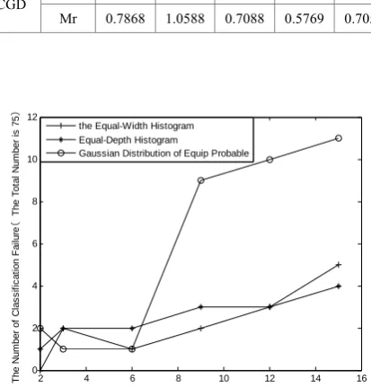
Figure 1. The Number of Estimating Failure (IRIS)
It shows that the accuracy is 97.43% when the number of the discrete regions is three by WH or the number of the discrete regions is four by CGD, and because of the number of test samples which cannot be classified is lager than that by CGD. Therefore the influence of failure rate is more than CGD from Table 3. We can see that the accuracies are respectively 87.33%,89.33% and 85.33% by WH, DH and CGD when the number of the discrete regions is three from Table 4. Although the accuracy is the highest by DH, the trend of decline by DH and CGD is obvious with increasing the number of the discrete regions. Failure rate is more than 30% when the number of the discrete regions is seven.
The results of estimating the missing variables discretized by WH, DH and CGD are shown in the Table 5. It shows average relative deviation and the maximal relative deviation of IRIS. The results of Ecoli are shown in Table 6. From Table 5 and Table 6, we can see that the average relative deviation and the maximal relative deviation have a gentle trend with increasing number of the regions.
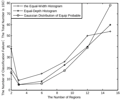
Estimating the missing values may fail by the inverse classification algorithm. Hence the number of test records which cannot be classified by the inverse classification algorithm should be considered when the average relative deviation and the maximal relative deviation are used to verify validity. The number of estimating failure with increasing number of the regions is illustrated in Figs.1 and 2. The number of estimating
f
ailure is directly proportional to the number of regions. The more the number of estimating failure, the less test samples reflected. Therefore estimating the missing values has little significance when the number of regions is lager than certain value.It shows that the number of estimating failures has the trend of rapid increase when the number of regions is lager than seven from Figs.1. It also has little significance when the number of regions is lager than certain value. Hence we study the three discrete methods when the number of regions are in certain range. Set the maximum regions is seven. The average relative deviation is the lowest by DH, and the maximal relative deviation is the
lowest by WH in Table 5. The average relative deviation and maximal relative deviation are both the lowest by WH in Table 6.
TABLEIV.
THE CLASSIFICATION RESULTS OF ECOLI
Regions 2 3 4 5 7
WH
A(%) 74.00 87.33 82.67 78.00 70.00
W(%) 26.00 12.00 12.67 14.00 8.67
F(%) 0.00 0.67 4.67 8.00 21.33
DH
A(%) 59.33 89.33 72.67 62.67 56.67
W(%) 40.67 10.67 21.33 16.67 8.00
F(%) 0.00 0.00 6.00 20.67 35.33
CGD
A(%) 80.00 85.33 81.33 74.67 58.00
W(%) 20.00 14.67 10.00 8.67 8.67
F(%) 0.00 0.00 8.67 1.67 33.33
TABLEVI.
THE ESTIMATING THE MISSING VALUES RESULTS OF ECOLI
Regions 2 3 4 5 7
WH Er 0.1665 0.1655 0.1772 0.1791 0.1925
Mr 0.6384 0.5392 0.7872 0.8269 0.8367
DH Er 0.1696 0.1713 0.1795 0.1974 0.1939
Mr 0.6384 0.5392 0.7872 0.8269 0.8367
CGD Er 0.1749 0.2697 0.2186 0.1885 0.2397
Mr 0.7868 1.0588 0.7088 0.5769 0.7059
TABLEV.
THE ESTIMATING THE MISSING VALUES RESULTS OF IRIS
Regions 2 3 4 5 7
WH Er 0.2103 0.2089 0.2107 0.2018 0.1905
Mr 0.7400 0.7400 0.7400 0.7400 0.7525
DH Er 0.2124 0.2109 0.1870 0.2062 0.1801
Mr 0.7400 0.7400 0.7933 0.7233 0.7803
CGD Er 0.2272 0.2067 0.1977 0.1990 0.1962
2 4 6 8 10 12 14 16 0
10 20 30 40 50 60 70 80
The Number of Regions
()
T
he Nu
m
be
r of
C
las
s
if
ic
a
ti
on F
ai
lur
e
T
he T
ot
a
l N
um
b
er
i
s
150 the Equal-Width Histogram
Equal-Depth Histogram
Gaussian Distribution of Equip Probable
Figure 2. The Number of Estimating Failure (Ecoli)
V. CONCLUSIONS
The inverse classification method of quantitative attributes is proposed to solve the limitations of discrete attributes. The inverse classification algorithm analyzes both the training samples and test samples. It also considers the class attributes of test sample. Firstly, a group of features are selected by using feature selection algorithm. Then, three discretization algorithms, WH, DH and CGD are used to convert the quantitative attributes into categorical form and construct the inverted statistics on the training data in order to analyze the training sample. Finally, the test data is analyzed in order to be classified by inverted statistics and to estimate the missing values by comparing the classification result with the desired class. The attributes are considered in estimating the missing values if classification result is the same as the desired class. Experiments on IRIS and Ecoli datasets respectively show that this method could find the class label effectively. The results of classification and estimating the missing values after discretization by WH are better. The classification result is better when the number of regions is approximately equal to the number of class labels.
REFERENCES
[1] Pendharkar P C, “A potential use of data envelopment analysis for the inverse classification problem,” Omega, Vol.30 (2002), pp. 243–248.
[2] Mannino M V, Koushik M, “The cost-minimizing inverse classification problem: a genetic algorithm approach,” Decision Support Systems Vol. 29(2000), pp. 283–300. [3] Aggarwal C C, Chen C, “The inverse classification problem,”
Journal of Computer Science and Technology Vol. 25(2010), pp. 1-11.
[4] Lin J, Keogh E, Lonardi S, Chiu B: Proceedings of 2003 8th, ACM SIGMOD, pp.2-11.
[5] Chakraborty B, “Feature Subset Selection by Particle Swarm Optimization with Fuzzy Fitness Function,” Proceedings of 2008 3rd ICISE, pp.1038-1042.
[6] Song L, “Study and Application of Multisensor Correlation
Analysis Methods,” Xi’an University of Science and