STATISTICAL ANALYSIS ON
ANGULAR DISTORTION OF WELDED
STRUCTURAL STEEL PLATES
P.Rajendran, V.R. Sivakumar, V.Gunaraj, Department of Mechanical Engineering, RVS College of Engineering and Technology,
Coimbatore- 641032, India.
V.VeL Murugan Sri Sakthi Engineering College Karamadai, Coimbatore - 641105, India.
ABSTRACT
Welding distortion during welding leads to dimensional inaccuracies and misalignments of structural members. In the butt welded plates angular distortion is particularly more pronounced among the different types of distortions. Non uniform transverse shrinkage along the depth of the welded plates is the cause of angular distortion. Distortion and residual stresses are largely opposed. Restriction of the angular distortion may lead to higher residual stresses. Prediction of angular distortion may help in reducing the distortion by providing initial angular distortion in the negative direction. Design of experiments (DOE) is a scientific approach of planning and conducting experiments to generate, analyze and interpretation of the data. In this study mathematical models were developed to predict angular distortion for a particular set of parameters. Using the mathematical equations trends of direct and indirect effects of the process variables on the angular distortion are presented in the graphical form and analyzed. This sensitively analysis helps in optimizing the welding process to improve the quality and life of the welded parts.
Keywords: Mathematical Models. Design of Experiments, Central Composite rotatable Design, Angular Distortion, Gas Metal Arc Welding.
INTRODUCTION
Gas metal are welding (GMAW) is the most extensively employed method of joining metal parts due to advantage of its speed, deep penetration and low spatter. Due to the highly localized transient heat input considerable residual stresses and deformations occur during and after welding. Deformations are classified into four categories (longitudinal shrinkage, bending deformation, transverse deformation and angular distortion).Angular distortion is particularly marked in the case of single side multi-pass but welding.
The extent of angular distortion depend on
1) The width and depth of the fusion zone relative to plate thickness 2) Type of joint
3) The weld sequence 4) Material properties and
5) The welding process control variables [1]
In this study, the statistical method of four factors, five level factorial central composite rotatable design has been used to develop mathematical models to correlate angular distortion with multi-pass process variables. The process variables considered are
1) Angle of electrode with work piece (), 2) Time gap between passes (t),
3) Wire feed rate (F) and 4) Welding speed (S)
Mathematical models are helpful in predicting the angular distortion under the influence of various process variables. This will be helpful in determining the angular distortion in the negative direction. So that after welding, angular distortion will be avoided Optimizations of welding process variables is also possible to minimize angular distortion.
Angular distortion () occurs at butt, lap, T and corner joints as a result of single –sided or also asymmetrical double – sided welding. The magnitude of angular distortion depends on the width and depth of the fusion zone relative to plate thickness, on the type of joint, on the weld pass sequence, on the thermo-mechanical material properties and on the characteristic parameters of the welding process [1]. Kumose et al. [2] have conducted some studies on how effectively elastic pre-straining could reduce the angular distortion of single pass fillet welding. Hirai and Nakamura [3] have conducted an investigation to determine the angular distortion as a function of plate thickness, wire feed rate and welding speed. Kihara and Masubuchi [4] have made an experimental investigation of how various welding process parameters, including the shape of the groove and the degrees of restraint, affect the angular change in butt welds. Five specimens with double-vee and single-vee groove were welded using multi-pass GMAW process and angular changes were measured and investigated. An extensive research work [5] conducted by ship building research association of Japan recommended the groove shape that minimizes the angular distortion.
Different heat source modeling developed with the help of Finite Element Analysis gives various magnitudes of angular distortion [1]. It is then difficult to predict experimental results and compare them with different practical cases. Hence the results predicted either by FEA analysis or by using mathematical models can serve as a certain approximation of the real one. Kuzminov [6] has developed a graph for angular distortion dependent on heat input per unit length of the weld and plate thickness. Mandal et al. [7] used statistical method of two level full factorial techniques to develop models, which correlate angular distortion with pulse MIG process variables and joint design parameters.
These developed models are very useful to determine quantitatively the angular distortion in the negative direction, so that after welding, angular distortion will not be there in the fabricated component. They are also useful for selecting optimum process variables for minimizing distortion in welded structures.
EXPERI MENTAL WORK
The experiments were designed based on five-level factorial central composite rotatable designs with full replications [8]. These experiments were conducted as per the design matrix using semiautomatic thyrister -controlled GMAW equipment. A servomotor-driven manipulator was used to maintain uniform welding speed. Copper-coated steel wire AWS ER70S-6 (BW-2), 1.2 mm diameter, in the form of coil was used, with CO2 as the shielding gas. Structural steel plate (IS: 2062) specimens 300 *150 *25 mm were welded together. Before the start of actual welding, the plates were tack welded at the ends. The tack welded plates were supported freely on a weld pad during welding.
PLAN OF INVESTIGATION
The plan was carry out the research in the following steps [8]:
3. Develop the design matrix.
4. Conduct the experiments as per the design matrix. 5. Record the responses, viz. Angular Distortion (). 6. Develop the mathematical model.
7. Test the significance of the coefficients, recalculating the value of the significant coefficients and arriving at the final mathematical model.
8. Test the adequacy of the mathematical model. 9. Validate the mathematical model.
10. Results and discussion
Identification of the Parameters
The following independently controllable process parameters were identified to carry out the experiments Angle of electrode with work piece ()
Time gap between passes (t) Wire feed rate(F) and Welding speed (S).
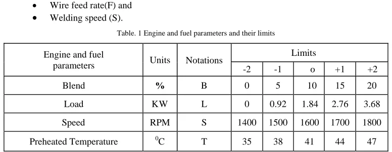
Table. 1 Engine and fuel parameters and their limits
Engine and fuel
parameters Units Notations
Limits
-2 -1 o +1 +2
Blend % B 0 5 10 15 20
Load KW L 0 0.92 1.84 2.76 3.68
Speed RPM S 1400 1500 1600 1700 1800
Preheated Temperature 0C T 35 38 41 44 47
Finding the Limits of the Fuel and Engine Parameters
Trial runs were carried out by varying one of the process parameters while keeping the rest of them at constant values [9]. The working range was decided upon by inspecting the bead for smooth appearance and the absence of any visible defects. The upper limit of the factor was coded as +2 and the lower limit as –2. The coded values for intermediate values were calculated from the following relationship:
max min
min max
2
2
X
X
X
X
X
X
i
--- (1)
Where Xi is the required coded value of a variable X; and X is any value of the variable from Xmin to Xmax. The selected process parameters with their limits, units, and notations are given in Table 1.
Table 1. Process variables and their levels (Four Factors – Five Levels)
Process parameters Units Notation
Limits
– 2 – 1 0 +1 +2
Angle of electrode to work piece Deg 70 80 90 100 110
Time gap between passes min t 5 10 15 20 25
Wire feed rate M min–1 F 5 5.25 5.5 5.75 6
Developing the Design Matrix
A five-level, three-factors, central composite rotatable factorial design |X], consisting of 31 sets of coded conditions is shown in Table 2. The design matrix comprises a full replication factorial design 23 [=8] plus six star points and six center points. All the welding parameters at the intermediate level (0) constitute center points and combinations at either it’s lowest (-2) or highest (+2) level with the other two parameters at the intermediate level constituting the star points. Thus the 31experimental runs allowed the estimation of the linear, quadratic and Two-way interactive effects of the process parameters on Angular Distortion.
Conducting the Experiment as per the Design Matrix
The experiments were conducted as per the design matrix at random, to avoid the possibility of systematic errors infiltrating the system.
Recording the Responses
Table.2. Design matrix and observed values of Angular Distortion
S. No. t F S
degrees
1 ‐1 ‐1 ‐1 ‐1 2.89
2 +1 ‐1 ‐1 ‐1 7.67
3 ‐1 +1 ‐1 ‐1 4.53
4 +1 +1 ‐1 ‐1 4.01
5 ‐1 ‐1 +1 ‐1 2.92
6 +1 ‐1 +1 ‐1 4.19
7 ‐1 +1 +1 ‐1 5.51
8 +1 +1 +1 ‐1 4.13
9 ‐1 ‐1 ‐1 +1 5.33
10 +1 ‐1 ‐1 +1 5.60
11 ‐1 +1 ‐1 +1 4.42
12 +1 +1 ‐1 +1 4.93
13 ‐1 ‐1 +1 +1 4.53
14 +1 ‐1 +1 +1 4.73
15 ‐1 +1 +1 +1 3.90
16 +1 +1 +1 +1 4.10
17 ‐2 0 0 0 3.73
18 +2 0 0 0 4.82
19 0 ‐2 0 0 3.87
20 0 2 0 0 4.10
21 0 0 ‐2 0 6.60
22 0 0 2 0 4.42
23 0 0 0 ‐2 3.55
24 0 0 0 2 3.33
25 0 0 0 0 3.99
26 0 0 0 0 4.73
27 0 0 0 0 4.60
28 0 0 0 0 3.90
29 0 0 0 0 4.70
30 0 0 0 0 4.74
Developing the Mathematical Model
The response function representing angular distortion can be expressed as = f (, t, F, S), and the relationship selected being a second-order response surface. The function is as follows
Where coefficients b1, b2, and b3 are linear terms, coefficients b11, b22, and b33 are second-order terms,
and coefficients b12, b13, and b23 are interaction terms.
Quality America -DOE PC IV. Software package [7] was used to calculate these coefficients. The mathematical model thus developed follows:
Testing the Significance of the Coefficients
The values of the coefficients give an idea to what extent the process parameters affect the responses quantitatively. In-significant coefficients were dropped along with the parameters with which they are associated, without affecting the accuracy of the model very much, this was carried out by conducting backward elimination analysis with t — probability criterion kept at 0.55 [7]. The significant coefficients were recalculated and the final mathematical model was developed using only these significant coefficients. The final mathematical model as determined by the above analysis is represented in the-following:
, (degrees) = 4.19 + 0.33 - 0.35 F – 0.15 2 – 0.29 t + 0.24 t F
– 0.11 t S + 0.12 F S (4)
Checking the Adequacy of the Model Developed
The adequacy of the model was tested using the analysis of variance techniques (ANOVA). As per this technique [8],
1) The calculated value of the F-ratio of the model developed should not exceed the standard tabulated value of F-ratio for a desired level of confidence (say 95%). and
2) If the calculated value of the R-ratio of the model developed exceeds the standard tabulated value of the R-ratio for a desired level of confidence (say 95%), then the model may be considered adequate within the-confidence limit. From Table 4, it is found that the model is adequate. Y = b0 + b1 + b2 t + b3 F + b4 S +b12 t + b13 F + b14 S + b23 t F + b24 t S + b34 F S +
b11 2
+ b22 t 2
+ b33 F 2
+ b44 S 2
(2)
= 4.53+0.33-0.04t-0.35F+0.009-0.152
+0.02t2+0.11F2+0.19S2-0.29t-0.06 F-0.11S+0.25tF-0.11tS+0.12FS
Table 3. Calculation of variance for testing the adequacy of the Model
Parameter Factors
(SS) df
Lack of fit
(SS) df
Error
Terms
(SS)
df F
ratio R ratio
Whether the
model is
adequate
Angular Distortion
(
)11.87 14 6.05 10 2.01 6 1.18 4.49 Adequate
F - Ratio = MS - l.ack of fit / MS - pure error R- Ratio = MS - factors / MS - pure error, Where. MS Mean Square - SS/df.
SS Sum of squares df - Degrees of freedom
F - Ratio (10,6,0.05)=4.06 and R - ratio (14,6,0.05)= 3.96
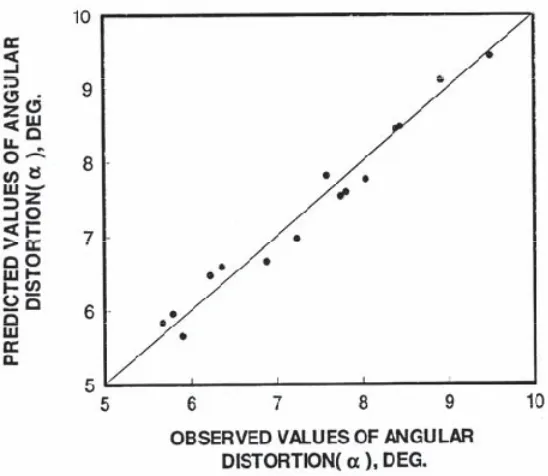
Validation of Mathematical Model
Validity of the developed models was tested by drawing scatter diagrams that show the observed and predicted values of angular distortion. A representative scatter diagram is shown in Fig. 1.
Fig. 1 Scatter Diagram for Angular Distortion.
RESULTS AND DISCUSSIONS
Direct effects of angle of electrode with work piece ()
Fig. 2 shows that the angular distortion increases with the increase in angle of electrode to work piece. The increase in angle of electrode results in preheating of work piece, which results in more penetration and width of the bead. An increase in the width of bead will contract more at the top surface of the weld pool and hence an increase in angular distortion is experienced. However slope of curve is initially more, but as increases the slope tends to decrease and becomes zero. This may be due to the fact that the effects of preheat decreases at higher values of , because increase in at higher values results in focusing axis of arc cone parallel to plate than towards the plate. Because of this width of bead decrease slightly, hence slope of increase in decreases at higher values of .
Direct effects of Time Gap Between Passes (t)
Figs. 3 represent the direct effect of time gap between passes (t) on final angular distortion (). From this figure, it is clear that decreases with the increase in t. When t is more, larger amount of heat is lost by the plate due to heat transfer and the plate temperature drops and reaches low as compared to that when t is less. So, partial amount of the heat applied to the plate during the next pass will be utilised in raising the plate temperature. Only the balance amount of heat applied is utilised for actual welding i.e. net amount of heat used for actual welding. As the width of bead decreases with the decrease in heat input, the angular distortion is less when t is more, because less bead width provides less contraction on the top of the bead.
Further, it is reported that the angular distortion may be determined by the following empirical relation [13]
= 2 T tan 2
Where = thermal expansion coefficient
T = maximum temperature of the material = groove angle.
When t is more, i.e. more time for cooling, the plate temperature drops to low as compared to that when t is less. In the above equation as T decreases the value of also decreases. The same trend is experienced here also.
Direct effects of Wire Feed Rate (F)
Figs. 4 depicts the direct effect of wire feed rate (F) on angular distortion (). From this it is clear that decreases from about 7.5 degrees to 5 degrees as F is increased from 4.5 to 6 m/min. For the same number of passes if F is increased, S is also increased to maintain the volume of metal deposited per unit length. Generally F has positive effect on (because increase in F will increase welding current and hence heat input also increases) and S has negative effect on . In this case, for the selected range of process variable, the negative effect of S on is predominant than the positive effect of F on when F is increased.
Artem Pilipenko [13] reported a relationship for angular distortion.
2
13
0
Sh
IV
.
Where I – Current, Amps.
V – Voltage, Volts.
S – Welding speed, m/sec.
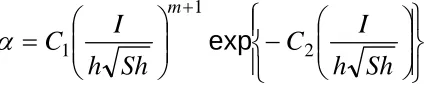
Watanabe and Satoh [14] reported another relationship for angular distortion.
Sh
h
I
C
Sh
h
I
C
m 2 1 1exp
Where C1, C2, m – constantsFrom these two equations, it is clear that the increase in welding speed results in decrease in the angular distortion. The same trend is experienced here also.
Direct effects of Welding Speed (S)
Welding speed is one of the main factor controlling heat input and the bead width. The bead width and dimensions of Heat Affected Zone (HAZ) decrease with the increase in S [9]. This is because heat input is inversely proportional to welding speed. Also, as per Christensen’s [15] empirical relationship between welding speed and HAZ dimensions, S has a negative effect on HAZ dimensions because of its influence on heat input. As width of the bead and HAZ dimensions decreases with the increase in welding speed, the angular distortion also decreases with the increase in S (Fig. 5).
Interaction Effects of Process Variables on Angular distortion
The difference in effect of one variable when a second variable is changed from one level to another level is known as interaction effects of process variables. The study of these interaction effects is very interesting and very useful for understanding the sensitivity of the process behaviour to the process control variables. However, the interaction effect of several variables at a time can be extremely complicated to analyse and have little significance. Hence an attempt had been made to analyse mainly the two-way interactive effects of the variables selected for investigation. Two-way interaction effects of process variables are also shown by three-dimensional contour plots.
Interaction effect of angle of electrode to work piece () and time gap between passes (t)
Fig. 6 shows the interaction effect of and t on . From the direct effects of and t on , it is found that has positive effect but t has negative effect on . From the figure it is obvious that increases from about 2 to 8 degrees with the increase in from 700 to 1100 for the value of t = 5 minutes. As the angle increases, the welding arc pre heats the metal and due to that width of bead increases (discussed in direct effect). At the same time, the time gap between passes is low and equal to 5 minutes; hence the work piece will be at higher temperature. It results in more amount of net heat input applied per unit length is used to increase the bead dimensions and due to that angular distortion increases. But as t is increased from 5 to 25 minutes, the rate of increase in with the increase in reduces gradually and the trend gets reversed for t = 25 minutes. This is because when the time gap between passes is more and equal to 25 minutes, the work piece is cooled to lower temperature and hence the net heat input is low. Hence, the bead width and the angular distortion reduces. It is also observed that the graphs intersect each other at = 900. This may be due to the transition of backhand welding to forehand welding at = 900.
These effects are further explained with the help of a response surface plot, as shown in Fig. 7. It is evident from the contour surface that, is maximum (about 8.5 degrees) when is at it’s higher (+2) and t is at its lower (-2) limits and is minimum (about 2.6 degrees) when both and t are at their lower limits.
Interaction effect of angle of electrode to work piece () and wire feed rate (F)
slope of the curve decreases with the increase in . At higher values of the nozzle-to-plate distance increases, hence slight decrease in the heat input result in decrease in the slope of the curve.
These effects are further discussed with the help of a response surface plot, as shown in Fig. 9. It is evident from the contour surface that, is maximum (about 7.5 degrees) when both and F are at their higher (+2) limits and is minimum (about 3.6 degrees) when both and F are at their lower limits.
Interaction effect of angle of electrode to work piece () and welding speed (S)
Fig.10 shows that increases with the increase in , for all the values of S. These effects are mainly due to the positive effect of on . However the values of is high (about 7 degrees) when the value of S = 8.4 cm/min and low (about 3 degrees) when the value of S = 10.8 cm/min. This may be due to the negative effect of S on weld bead. This is because heat input is inversely proportional to welding speed (as discussed in direct effect). However the slope of the curve decreases with the increase in beyond 900. Even though the pre-heating of plate is experienced when is increased beyond 900, at higher welding speed, the effect of pre-heating is less. At the same time increase in beyond 900 results in focussing of axis of the arc cone parallel to the plate than towards the plate, hence bead width decreases slightly [31] and thus the slope of . The slope becomes almost zero at = 1100.
These effects are further explained with the help of a response surface plot, as shown in Fig. 11. It is evident from the contour surface that, is maximum (about 7.5 degrees) when is at higher (+2) limits and S is at either lower (-2) limit or at higher (+2) limit. The value is minimum (about 4.6 degrees) when is at lower (-2) limit and S at (0) limit.
Interaction effect of time gap between passes (t) and Welding Speed (S)
Fig.12 shows the interaction effects of t and S on . From the fig, it is apparent that decreases with the increase in t for all values of S. The negative effect of S on is higher at lower value of t, however this negative effect of S on gradually decreases as t is increased from 5 min to 25 min. This may be due to the fact that the decrease rate is more at lower level of S compared to that of at higher level as explained in the direct effect. Also the combined negative effect of t and S on makes the curve steeper at lower level of S.
These effects are further explained with the help of a response surface plot, as shown in Fig.13. It is evident from the contour surface that, is maximum (about 8.5 degrees) when both S and t were at lower (-2) limits and is minimum (about 4.3 degrees) when both S and t were at higher (+2) limit.
Interaction effect of Wire Feed Rate (F) and Welding Speed (S)
Fig. 14 shows the interaction effects of F and S on . From the direct effects of F and S on , it was found both F and S had negative effect on . However in the interaction effect, the slope of the curve showing decreasing trend of with increase in S. This might be due to the fact that the decrease rate of is higher at lower level of S (-2 level) compared to that of at higher level (+2 level) as explained in direct effect. Also the negative effect of S on at lower level of S (-2 level) gradually changed to positive effect at higher level of S (+2 level).
These effects are further explained with the help of a response surface plot, as shown in Fig. 15. It is evident from the contour surface that, is maximum (about 7.5 degrees) when S and F were at lower (-2) limits and is minimum (about 5 degrees) when S is at its (0) limit and F is at its higher (+2) limit.
Conclusions
The conclusions below were arrived at from this investigation.
All the models developed are simple quadratic equations of first and second order relating welding variables with weld strength parameters and therefore can be easily utilized for predicting these parameters for any given set of process variables.
Angular distortion increased by 2.1 degrees as angle of electrode with work piece was increased from 70 deg to 110 deg
The process variables time gap between passes, wire feed rate and welding speed had negative effect on angular distortion.
Angular distortion decreased by 1.9 degrees as time gap between passes increased from 5 min to 25 min
Angular distortion decreased by 1.9 degrees as wire feed rate increased from 5 m/min to 6 m/min
Angular distortion decreased by 1.3 degrees as welding speed increased from 8.4 cm/min to 10.8 cm/min
All the process variables had a strong interaction effect on angular distortions.
Fig.2 Direct Effect of Angle of Electrode with Work Piece on Angular Distortion.
Fig3. Direct Effect of Time Gap between Passes on Angular Distortion.
70(-2) 80(-1) 90(0) 100(+1) 110(+2) . 4 5 6 7 A n g u la r d is to rt ion ( ) , d e g
Angle of electrode with work piece ( ), deg t=15 min
F=5.5 m/min S=8.6 cm/min
5(-2) 10(-1) 15(0) 20(+1) 25(+2) . 3.5 4.5 5.5 6.5 A n g u la r d is to rt io n ( ), d e g
Time gap between passes (t), min
Fig.4 Direct Effect of Wire Feed Rate on Angular Distortion.
Fig.5 Direct Effect of Welding Speed on Angular Distortion.
5(-2) 5.25(-1) 5.5(0) 5.75(+1) 6(+2) . 4
5 6 7 8
A
n
g
u
la
r
d
is
to
rt
io
n
(
),
d
e
g
W ire feed rate (F), m/min
=90 deg
t=15 min S=8.6 cm/min
8.4(-2) 9(-1) 9.6(0) 10.2(+1) 10.8(+2) . 5
6 7
W elding speed (S) cm/min
=90 deg
t=15 min F=5.5 m/min
A
n
g
u
la
r
d
is
to
rt
io
n
(
),
d
e
Fig.6. Interaction Effect of Angle of Electrode with Work Piece and Time Gap between Passes on Angular distortion.
Fig.7. Response surface for Interaction Effect of Angle of Electrode with Work Piece and Time Gap between Passes on Angular distortion. 70(-2) 80(-1) 90(0) 100(+1) 110(+2) .
1.5 3.5 5.5 7.5 9.5
Angle of electrode with work piece ( ), DEG F=5.5 m/min
S=9.6 cm/min t=5 min
t=10 min
t=15 min
t=20 min
t=25 min
A
n
g
u
la
r
d
is
to
rt
io
n
(
),
d
e
g
F&S at +2 level
F&S at -2 level
Fig.8.Interaction Effect of Angle of Electrode with Work Piece and Wire Feed Rate on Angular distortion.
Fig.9.Response surface for Interaction Effect of Angle of Electrode with Work Piece and Wire Feed Rate on Angular distortion.
70(-2) 80(-1) 90(0) 100(+1) 110(+2) . 3
4 5 6 7 8
t=15 min
S=9.6 cm/min F=6 m/min
F=5.75 m/min
F=5.5 m/min
F=5.25 m/min F=5 m/min
A
n
g
u
la
r
d
is
to
rt
io
n
(
),
d
e
g
Angle of electrode with work piece ( ), DEG
t&S at +2 level
t&S at -2 level
Fig.10.Interaction Effect of Angle of Electrode with Work Piece and Welding Speed on Angular distortion.
Fig.11.Response surface for Interaction Effect of Angle of Electrode with Work Piece and Welding Speed on Angular distortion. 70(-2) 80(-1) 90(0) 100(+1) 110(+2) .
4 5 6 7
t=15 min F=5.75 m/min
S=9.6 cm/min S=9 &10.2 cm/min S=8.4 &10.8 cm/min
A
n
g
u
la
r
d
is
to
rt
io
n
(
)
,
d
e
g
Angle of electrode with work piece ( ), DEG
t&F at +2 level
t&F at -2 level
Fig.12.Interaction Effect of Time Gap between Passes and Welding Speed on Angular distortion.
Fig.13. Response surface for Interaction Effect of Time Gap between Passes and Welding Speed on Angular distortion. 0 5(-2) 10(-1) 15(0) 20(+1) 25(+2) 30
4 5 6 7 8 9
Time gap between passes ( t ), min
=90 deg
F=5.5 m/min S=8.4 cm/min
S=9 cm/min
S=9.6 cm/min
S=10.2 cm/min
S=10.8 cm/min
A
n
g
u
la
r
d
is
to
rt
io
n
(
),
d
e
g
&F at +2 level
&F at -2 level
Fig.14.Interaction Effect of Wire Feed and Welding Speed on Angular distortion.
Fig.15.Response surface for Interaction Effect of Wire Feed and Welding Speed on Angular distortion.
References
[1] Vinokurov, V. A. 1977. Welding Stresses and Distortion. Wetherby. British Library.
[2] Kumose, T., Yoshida, T., Abe, T., and Onoue, H. 1954. Predictions of angular distortion caused by one pass fillet welding. Welding Journal 33: 945–956.
[3] Hirai, S., and Nakamura, I. 1955. Research Ishikawajima Review, pp. 59–68.
[4] Kihara, H., and Masubuchi, K. 1956. Studies on the shrinkage and residual welding stress of constrained fundamental joint. Report No. 24, Transportation Technical Research Institute, No. 7.
[5] ”Researches on weld procedures of thick steel plates used in the construction of large size ships”. Report of Ship building research association of Japan, 26, 1959.
[6] Kuzinov,A.S “ Calculation principles of total ship hall structures” Central scientific research institute of ship building industry, Russia N9,1956.
[7] Mandal, A., and Parmar, R. S. 1997. Effect of process variables and angular distortion of pulse GMAW welded HSLA plates. Indian Welding Journal, pp. 26–34.
[8] Cochran, W. G., and Cox, G. M. 1963. Experimental Designs. India, Asia Publishing House.
[9] Gunaraj, V., and Murugan, N. 2002. Prediction of heat-affected zone characteristics in submerged arc welding of structural steel plates. Welding Journal 81(3): 45-s to 53-s.
[10] Murugan, N., and Parmar, R. S. 1994. Effects of MIG process parameters on the surfacing of stainless steel. Journal of Materials Processing Technology 41: 381–398.
[11] DOE — PC IV. 1998. Software reference manual, Quality America, Inc.
[12] Gunaraj, V., and Murugan, N. 1999. Application of response surface methodology for predicting weld bead quality in submerged arc welding of pipes. Journal of Materials Processing Technology 88: 266–275.
5(-2) 5.25(-1) 5.5(0) 5.75(+1) 6(+2) . 4.5
5.5 6.5 7.5
8.5 S=8.4 cm/min t=15 min=90 deg
S=9.6 cm/min S=9 cm/min
S=10.2 cm/min S=10.8 cm/min
A
n
g
u
lar
d
is
to
rt
io
n
(
)
,
d
e
g
W ire feed rate (F), m/min
&t at +2 level
&t at -2 level
[13] Pilipencko A. 2001. Computer simulation of residual stresses and distortion of thick plates in multi-electrode submerged arc welding — Their mitigation techniques. PhD thesis, Norwegian University of Science and Technology, Norway.
[14] Watanabe, M., and Satoh, K. 1961 Effect of welding conditions on the shrinkage and distortion in welded structures. Welding Journal
40(8): 377-s to 384-s.