Simpler, Faster, and More Robust T-test Based Leakage Detection

Simpler, Faster, and More Robust

T-test Based Leakage Detection

A. Adam Ding1, Cong Chen2, and Thomas Eisenbarth2

1

Northeastern University, Boston, MA, USA

{a.ding}@neu.edu

2

Worcester Polytechnic Institute, Worcester, MA, USA

{cchen3,teisenbarth}@wpi.edu

Abstract. The TVLA procedure using the t-test has become a popu-lar leakage detection method. To protect against environmental fluctua-tion in laboratory measurements, we propose a paired t-test to improve the standard procedure. We take advantage of statistical matched-pairs design to remove the environmental noise effect in leakage detection. Higher order leakage detection is further improved with a moving av-erage method. We compare the proposed test with standard t-test on synthetic data and physical measurements. Our results show that the proposed tests are robust to environmental noise.

1

Motivation

More than 15 years after the proposal of DPA, standardized side channel leakage detection is still a topic of controversial discussion. While Common Criteria (CC) testing is an established process for highly security critical applications such as banking smart cards and passport ICs, the process is slow and costly. While appropriate for high-security applications, CC is too expensive and too slow to keep up with the innovation cycle of a myriad of new networked embedded products that are currently being deployed as the Internet of Things. As a result, an increasing part of the world we live in will be monitored and controlled by embedded computing platforms that, without the right requirements in place, will be vulnerable to even the most basic physical attacks such as straightforward DPA.

Due to its simplicity, it is applicable to a fairly wide range of cryptographic implementations. In fact, academics have started to adopt this test to provide ev-idence of existing leakages or their absence [1, 3–5, 12, 14, 15, 19]. With increased popularity, scrutiny of the TVLA test has also increased. Mather et al. [13] studied the statistical power and computation complexity of the t-test versus mutual information (MI) test, and found that t-test does better in the majority of cases. Schneider and Moradi [18] for example showed how the t-test higher order moments can be computed in a single pass. They also discussed the tests sensitivity to the measurement setup and proposed a randomized measurement order. Durveaux and Standaert [8] evaluate the convenience of the TVLA test for detecting relevant points in a leakage trace. They also uncover the implica-tions of good and bad choices of the fixed case for the fixed-vs-random version of the TVLA test and discuss the potential of a fixed-vs-fixed scenario.

However, there are other issues besides the choice of the fixed input and the measurement setup that can negatively impact the outcome for the t-test based leakage detection. Environmental effects can influence the t-test in a neg-ative way, i.e., will decrease its sensitivity. In the worst case, this means that a leaky device may pass the test only because the environmental noise was strong enough. This is a problem for the proposed objective of the TVLA test, i.e. self-certification by non-professionals who are not required to have a broad background in side channel analysis.

Our Contribution In this work, we propose the adoption of the paired t-test for leakage detection, especially in cases where long measurement campaigns are performed to identify nimble leakages. We discuss several practical issues of the classic t-test used in leakage detection and show that many of them can be avoided when using the paired t-test. To reap the benefits of the locality of the individual differences of the paired t-test in the higher order case, we further propose to replace the centered moments with a local approximation. These approximated central moments are computed over a small and local moving window, making the entire process a single-pass analysis. In summary, we show that

– the paired t-test is more robust to environmental noise such as tempera-ture changes and drifts often observed in longer measurement campaigns, resulting in a faster and more reliable leakage detection.

– using moving averages instead of a central average results in much better performance for higher order and multivariate leakage detection if common measurement noise between the two classes of traces is present, while intro-ducing a vanishingly small inaccuracy if no such common noise appears. The improvement of the moving averages applies both to the paired and unpaired t-tests.

2

Background

In the framework of [9], the potential leakage for a device under test (DUT) can be detected by comparing two sets of measurementsLAandLB on the DUT. A

popular test for the comparison is Welch’s t-test, which aims to detect the mean differences between the two sets of measurements. The null hypothesis is that the two samples come from the same population so that their population means µAandµB are the same. Let ¯LAand ¯LBdenote their sample means,s2Aands2B

denote their sample variance, nA and nB denote the number of measurements

in each set. Then the t-test statistic and its degree of freedom are given by

tu=

¯ LA−L¯B

q

s2

A

nA +

s2

B

nB

, v= (

s2_A

nA +

s2_B

nB)

2

(s

2

A nA)2

nA−1 +

(s

2

B nB)2

nB−1

. (1)

The p-value of the t-test is calculated as the probability, under a t-distribution with v degree of freedom, that the random variable exceeds observed statistic

|tu|. This is readily done in Matlab as 2∗(1−tcdf(·, v)) and in R as 2∗(1−

qt(·, df =v)). The null hypothesis of no leakage is rejected when the p-value is smaller than a threshold, or equivalently when the t-test statistic|tu|exceeds a

corresponding threshold. The rejection criterion of |tu|>4.5 is often used [18,

9]. Since P r(|tdf=v>1000|>4.5)<0.00001, this threshold leads to a confidence level>0.99999.

For leakage detection, aspecifict-test use two setsLAandLB corresponding

to different values of an intermediate variable:V =vAandV =vB. To avoid the

dependence on the intermediate value and the power model, non-specifict-test often uses the fixed versus random setup. That is, the first set LA is collected

with a fixed plaintext xA, while the second set LB is collected with random

plaintexts xB drawn from the uniform distribution. Then if there is leakage

through an (unspecified) intermediate variableV, then

LA=V(k, xA) +rA LB=V(k, xB) +rB, (2)

wherek is the secret key,rA andrB are random measurement noises with zero

means and variance σ2

A and σB2 respectively. The non-specific t-test can detect

the leakage, with large numbers of measurements nA and nB, when the fixed

intermediate state V(k, xA) differs from the expected value of the random

in-termediate stateExB[V(k, xB)] where the expectation is taken over the uniform

random plaintextsxB.

0 2000 4000 6000 8000 10000 1050

1100 1150 1200 1250 1300 1350 1400

Power Consumption

Fixed average (Window size=100)

Fig. 1. Power consumption moving averages at a key-sensitive leakage point on the DPAv2 template traces

3

Methodology

This section introduces paired t-test and shows its superiority in a leakage model with environmental noise. The paired t-test retains its advantage of being a straightforward one-pass algorithm by making use of moving or local averages. By relying on the difference of matched pairs, the method is inherently numeri-cally stable while retaining computational efficiency and parallelizability of the original t-test.

3.1 Paired T-Test

Welch’s t-test works well when the measurement noisesrA andrB are

indepen-dent between the two sets of measurements. However, two sets of measurements can also share common variation sources during a measurement campaign. For example, power consumption and variance may change due to common envi-ronmental factors such as room temperature. While these envienvi-ronmental factors usually change slowly, such noise variation is more pronounced over a longer time period. With hard to detect leakages, often hundreds of thousands to millions of measurement traces are required for detection. These measurements usually take many hours and the environmental fluctuation is of concern in such situations. For example, for the DPA V2 contest, there are one million template traces collected over 3 days and 19 hours, which show a clear temporal pattern [10]. Figure 1 (a subgraph of Figure 2 in [10]) shows the average power consump-tion at 2373-th time point on the traces of DPAv2, using mean values over 100 non-overlapping subsequent traces.

D =LA−LB. The paired difference cancels the noise variation from the

com-mon source, making it easier to detect nonzero population difference. The null hypothesis ofµA=µB is equivalent to that the mean differenceµD= 0, which

is tested by a paired t-test. Let ¯D ands2

D denote the sample mean and sample

variances of the paired differencesD1, ...,Dn. The paired t-test statistic is

tp=

¯ D

q

s2

D

n

, (3)

with the degree of freedomn−1. The null hypothesis of non-leakage is rejected when|tp|exceeds the threshold of 4.5.

To quantify the difference between the two versions of t-test, we can compare the paired t-test (3) and the unpaired t-test (1) here withnA=nB=n.

First, without common variation sources under model (2),V ar(D) =V ar(LA)+

V ar(LB) = ˜σ2A+˜σ2B. Here ˜σ2A=σ2A+V ar[V(k, xA)] and ˜σ2B=σB2+V ar[V(k, xB)].

Notice that ¯D= ¯LA−L¯B, so for largen, the paired t-test and unpaired t-test are

equivalent withtu ≈tp ≈( ¯LA−L¯B)/

p

(˜σ2

A+ ˜σ2B)/n. The paired t-test works

even if the two group variances are unequal ˜σ2_A 6= ˜σ_B2. The two versions of the t-test perform almost the same in this case.

However, the paired t-test detects leakage faster if there are common noise variation sources. To see this, we explicitly model the common environmental factor induced variation not covered by model (2).

LA=V(k, xA) +rA+rE LB=V(k, xB) +rB+rE, (4)

whererEis the noise caused by common environmental factors, with mean zero

and varianceσE. TherAandrBhere denote the random measurement noises

ex-cluding common variations so thatrAandrB are independent, with zero means

and varianceσ2

Aandσ2Brespectively. Again we denote ˜σ2A=σ2A+V ar[V(k, xA)]

and ˜σ2

B = σ

2

B +V ar[V(k, xB)]. Then tu ≈ ( ¯LA−L¯B)/

p

(˜σ2

A+ ˜σ

2

B+ 2σ

2

E)/n

whiletp≈( ¯LA−L¯B)/

p

(˜σ_A2 + ˜σ2_B)/n. The paired t-test statistic|tp|has a

big-ger value than the unpaired t-test|tu|, thus identifies the leakage more efficiently.

The difference increases when the environmental noise σE increases. Hence, the

paired t-test performs as well or better than the unpaired test. However, the matched-pairs design of the paired t-test cancels common noise found in both pairs, making the test more robust to suboptimal measurement setups and en-vironmental noise.

3.2 Higher Order and Multivariate Leakage Detection

The t-test can also be applied to detect higher order leakage and multivariate leakage [9, 18]. For d-th order leakage at a single time point, the t-test compares sample means of (LA−L¯A)dand (LB−L¯B)d. Under the matched-pairs design,

the paired t-test would simply work on the difference

to yield the test statistic (3): tp = ¯D/

p

s2

D/n. Multivariate leakage combines

leakage observation at multiple time points. Ad-variate leakage combines leakage L(1)_{, ...,L}(d)_{at thedtime pointst}

1, ...,tdrespectively. The combination is done

through the centered product CP(L(1)_{, ..., L}(d)_{) = (L}(1)_−L¯(1)_)(L(2) _−L¯(2)_)·

· ·(L(d)_−L¯(d)_{). The standard d-variate leakage detection t-test compares the} sample means ofCP(L(1)_A , ..., L(_Ad)) andCP(L(1)_B , ..., L(_Bd)) with statistic (1). The paired t-test (3) uses the differenceD= [CP(L(1)_A , ..., L(_Ad))−CP(L(1)_B , ..., L(_Bd))] .

However, these tests (including the paired t-test) do not eliminate environ-mental noise effects on the higher order and multivariate leakage detection. The centering terms (the subtracted ¯L) in the combination function also need adjust-ment due to environadjust-mental noises, which are not random noise but follow some temporal patterns. To see this, we use the bivariate leakage model for first-order masked device as an example.

The leakage measurements at the two time pointst1 andt2 leak two inter-mediate values V(1)_{(k, x, m) andV}(2)_{(k, x, m) where k, xand mare the secret} key, plaintext and mask respectively. For uniformly distributedm,V(1)(k, x, m) and V(2)(k, x, m) both follow a distribution not affected by k and x, there-fore no first order leakage exits. Without loss of generality, we assume that Em[V(1)(k, x, m)] =Em[V(2)(k, x, m)] = 0, and the second order leakage comes

from the product combinationV(1)V(2). [17] derived the strongest leakage com-bination function under a second order leakage model without the environmental noises:

L(1)=c(1)+V(1)(k, x, m) +r(1), L(2) =c(2)+V(2)(k, x, m) +r(2), (6)

wherer(1)_andr(2)_{are zero-mean random pure measurement noises with variance} σ2

1 and σ22 respectively. Under model (6), [17] showed that centered product leakage (L(1)_−c(1)_)(L(2)_−c(2)_{) is the strongest. Sincec}

1 and c2 are unknown in practice, they are estimated by ¯L(1) _{= ¯c}(1)_{+ ¯V}(1)_{+ ¯r}(1) _{and ¯L}(2) _{= ¯c}(2)₊

¯

V(2)_{+ ¯r}(2)_{. With large number of traces, ¯L}(1)_≈c¯(1)_{and ¯L}(2)_≈¯c(2)_{by the law of} large number. Hence (L(1)_−L¯(1)_)(L(2)_−L¯(2)_{) approximate the optimal leakage} (L(1)_−c(1)_)(L(2)_−c(2)_{) well. However, considering environment induced noises,} this is no longer the strongest leakage combination function. Let us assume that

L(1)=c(1)+V(1)(k, x, m)+r(1)+r_E(1), L(2)=c(2)+V(2)(k, x, m)+r(2)+r(2)_E , (7)

where r(1)_E and r(2)_E are environment induced noises which has mean zero but follow some temporal pattern rather than being random noise. The optimal leakage then becomes (L(1)_−c(1)_−r(1)

E )(L

(2)_−c(2)_−r(2)

E ) instead. Therefore,

we propose that the centering means ¯L(1) _{and ¯L}(2) _{are calculated as moving} averages from traces with a window of sizenw around the trace to be centered,

rather than the average over all traces. The temporal patterns for r_E(1) andr_E(2), such as in Figure 1, are usually slow changing. Hence, for a moderate window size, saynw= 100, the moving averages ¯L(1)≈c(1)+r

(1)

E and ¯L

(2)_≈c(2)_+r(2)

When there are no environment induced noises r_E(1) and r(2)_E , using bigger window size nw can improve the precision. However, comparing to centering

on averages of all traces, we can prove that centering the moving averages only losesO(1/nw) proportion of statistical efficiency under model (6). More precisely,

denote the theoretical optimal leakage detection statistic as

∆= (L(1)_A −c(1))(L(2)_A −c(2))−(L(1)_B −c(1))(L(2)_B −c(2)). (8)

And denote the leakage detection statistic using moving average of a window sizenw as

D= (L(1)_A −L¯(1)_A )(L(2)_A −L¯(2)_A )−(L(1)_B −L¯(1)_B )(L(2)_B −L¯(2)_B ). (9)

Then for large sample size n, the t-test statistic (3) is approximately tp(D)≈

E(D)/pV ar(D)/n, and the optimal leakage detection t-test statistic is approx-imately tp(∆) ≈ E(∆)/

p

V ar(∆)/n. A quantitative comparison of these two statistic is given in the next Theorem.

Theorem 1 Under the second-order leakage model (6), E(D)

p

V ar(D)/n

p

V ar(∆)/n E(∆) = 1−

η nw

+O( 1 n2

w

), (10)

where the factor η is given by

η= _{V ar}1_(∆)[V ar(V_A(1))V ar(V_A(2)) +V ar(V_B(1))V ar(V_B(2)) +E2_(V(1)

A V

(2)

A )

+E2_(V(1)

B V

(2)

B )−V ar(V

(1)

A V

(2)

A )−V ar(V

(1)

B V

(2)

B )].

The proof of Theorem 1 is provided in Appendix A.

The factorη is usually small. When the noise variances σ2

1 and σ22 are big (so that the leakage is hard to detect), this factor η = O[1/(σ2

1σ22)] ≈ 0. For practical situations, oftenη <1. Hence using, say,nw = 100 make the leakage

detection statistic robust to environmental noises r_E(1) and r(2)_E , at the price of a very small statistical efficiency loss when no environmental noises exist. Therefore, we recommend this paired moving-average based t-test (MA-t-test) over the existing tests.

We can also estimate the optimal window sizenw with some rough ideas of

environmental noise fluctuation. The potential harm in using too wide a window is to introduce bias in the estimated centering quantities. Let the environmental noise be described as rE(t) for the t = 1,2, ..., T traces, and P

T

t=1rE(t) = 0.

Then the environmental noise induced bias in the moving average is bounded as b ≤a0n2w/2 where a0 is the maximum of the derivative |rE0 (t)|. Let∆∗b denote

the test statistic in equation (8) where the centering quantitiesc(1) _andc(2) _are each biased by the amountb. Then, (see Appendix B),E(∆∗_b) =E(∆) and

V ar(∆∗_b) V ar(∆) = 1 +

b2_η∗

V ar(∆)+o(n 4

w)≤1 +

a2 0n4wη∗

4V ar(∆)+o(n 4

bounds the harm of using a too big nwvalue, whereη∗ is

V ar(L(1)_A ) +V ar(L(2)_A ) +V ar(L(1)_B ) +V ar(L_B(2)) + 2E(V_A(1)V_A(2)) + 2E(V_B(1)V_B(2)).

Matching the equations (11) and (10), we can estimate the optimal window size fromn5w≈

4[V ar(V_A(1))V ar(V_A(2)) +V ar(V_B(1))V ar(V_B(2)) +E2(V_A(1)V_A(2)) +E2(V_B(1)V_B(2))] a2

0[V ar(L (1)

A ) +V ar(L

(2)

A ) +V ar(L

(1)

B ) +V ar(L

(2)

B ) + 2E(V

(1)

A V

(2)

A ) + 2E(V

(1)

B V

(2)

B )]

.

As an example, we estimate this window size using parameters for data sets reported in literature. For the 2373-th time point on the traces on the DPA V2 contest data shown in Figure 1, the environmental fluctuation is approximately four periods of sinusoidal curve over one million traces with magnitude ≈100. Soa0≈1/400. For simplicity, we assume that both leakage time points follow a similar power model for the shown data, so that the noise variancesσ1=σ2≈ 300. That is, V_A(i) = HWi, i = 1,2, with HWi as hamming weights related

to masks and plaintexts as in the model of [17, 7]. The with the signal-noise-ratio around 0.1 [7],≈30. For one byte hamming weights model,V ar(V_A(1))≈

302(2) = 1800. Hence the optimal window size here is ≈ [4002×4×18002×

2/(3002 ×4)]1/5 ≈ 30 traces. This optimal window size does vary with the magnitude of the environmental fluctuation and the leakage signal-noise-ratio which are not known to a tester as a prior. But this example can serve as a rough benchmark, and a window size of a few dozens may be used in practice.

3.3 Computational Efficiency

The paired t-test also has computational advantages over Welch’s t-test. As pointed out in [18], computational stability can become an issue when using raw moments for large measurement campaigns. The paired t-test computes mean

¯

D and variances2_Dof local differencesD. In case there is no detectable leakage, LA andLB have the same mean. Hence, the differencesD are mean-free3. Even

computing ¯D= 1 ni

P

di is thus numerically stable. The sample variances2Dcan

be computed as s2_D = D2_{−( ¯D)}2_{, where only the first term D}2 _{is not} mean-free. We used the incremental equation from [16, eq. (1.3)] to avoid numerical problems. Moreover, by applying the incremental equation for ¯Das well, we were able to exploit straightforward parallelism when computing ¯D and variances2

D.

The situation essentially remains the same for higher order or multivariate analysis: The differences D are still mean-free in the no-leakage case. Through the use of local averages, the three-pass approach is not necessary, since moving averages are used instead of global averages (cf. eq. (9)). Computing moving

3

Table 1. Computation Accuracy between our incremental method and Two-pass al-gorithm

1st order 2nd order 3rd order 4th order 5th order

Our method 50.0097 2.4679e+3 4.5981e+5 7.3616e+7 1.7974e+10

Two Pass 50.0097 2.4679e+3 4.5981e+5 7.3616e+7 1.7974e+10

averages is a local operation, as only nearby traces are considered. When pro-cessing traces in large blocks of e.g. 10k traces, all data needed for local averages is within the same file and can easily be accessed when needed, making the al-gorithm essentially one-pass. Similarly as in [18], we also give the experimental results using our method on 100 million simulated traces with ∼ N(100,25). Specifically, we compute the second parameterss2

D using the difference leakages:

D=LA−LBfor first order test whileD= [(LA−L¯A,nw)

d_−(L

B−L¯B,nw)

d_{] for}

d-th order tests with moving average of window size nw = 100. Table 1 shows

our method matches the two-pass algorithm which computes the mean first and then the variance of the preprocessed traces. Note thatDis not normalized using the central momentCM2 and thus the second parameter is significantly larger than that in [18]. In the experiments, the same numerical stability is achieved without an extra pass, by focusing on the difference leakages.

4

Experimental Verification

To show the advantages of the new approach, the performances of the paired t-test (3) and the unpaired t-test (1) on synthetic data are compared.

First, we generate data for first order leakage according to model (4), where the environmental noiserEfollows a sinusoidal pattern similar to Figure 1. The

sinusoidal period is set as 200,000 traces, and the sinusoidal magnitude is set as the pure measurement noise standard deviation σA = σB = 50. Hamming

weight (HW) leakage is assumed in model (4). The first group A uses a fixed plaintext input corresponds toHW = 5, while the second group B uses random plaintexts. The paired t-test (3) and the unpaired t-test (1) are applied to the first n = 30000,60000, ...,300000 pairs of traces. The experiment is repeated 1000 times, and the proportions of leakage detection (rejection by each t-test) are plotted in Figure 2.

Without any environmental noiserE, the paired and unpaired t-tests perform

the same. Their success rate curves overlap each other. With the sinusoidal noise rE, the unpaired t-test uses many more traces to detect the leakage, while the

paired t-test does not suffer from such performance degradation.

Notice that the environmental noiserE often changes slowly as in Figure 1.

Hence, its effect is small for easy to detect leakage, when only a few hundreds or a few thousands of traces are needed. However, for hard to detect leakage, the effect has to be considered. We set a high noise levelσA=σB = 50 to simulate a DUT

Fig. 2.T-test comparison for 1O leakage with and without a sinusoidal driftrE.

Second, we also generate data from the 2nd-order leakage model (7). The noise levels at the two leakage points, for both groups A and B, are set as σ1 = σ2 = 10 which are close to the levels in the physical implementation reported by [7]. We use the same sinusoidal environmental noise rE as before.

The first group A uses a fixed plaintext input corresponds toHW = 1, while the second group B uses random plaintexts. The proportions of leakage detection are plotted in Figure 3. Again, we observe a serious degradation of t-test power to

Fig. 3.T-test comparison for 2O leakage with a sinusoidal driftrE.

detect the leakage, when the environmental noiserEis present. The paired t-test

rE. That is due to the incorrect centering quantity for the 2O test as discussed

in Section 3.2. Using the proposed method of centering at the moving average with window size 100, the paired MA-t-test has a performance close to the case where all environmental noiserE is removed.

5

Practical Application

To show the advantage of the paired t-test in real measurement campaigns, we compare the performances of the unpaired and paired t-tests when analyzing an unprotected and an protected hardware implementation. The analysis focuses on the non-specific fixed vs. random t-test. We apply both tests to detect the first order leakage in the power traces acquired from an unprotected implementation of the NSA lightweight cipher Simon [2]. More specifically, a round-based imple-mentation of Simon128/128 was used, which encrypts a 128-bit plaintext block with a 128-bit key in 68 rounds of operation. The second target is a masked engine of the same cipher. It is protected using three-share Threshold Imple-mentation (TI) scheme, which is a round based variant of the TI Simon engine proposed in [19].

Both implementations are ported onto the SASEBO-GII board for power trace collection. The board is clocked at 3MHz and a Tektronix oscilloscope samples the power consumption at 100MS/s. Since Simon128/128 has 68 rounds, one power trace has about 68× 1

3M Hz×100M S/s≈2300 time samples to cover

the whole encryption and hence in the following experiments 2500 samples are taken in each measurement. The measurement setup is a modern setup that features a DC block and an amplifier. Note that the DC block will already take care of slow DC drifts that can affect the sensitivity of the unpaired t-test, as shown in Section 4. However, the DC block does not affect variations of the peak-to-peak height within traces, which are much more relevant for DPA. As the following experiments show, the paired t-test still shows improvement in such advanced setups.

5.1 Solving the Test-Order Bias

as the random selection method. Experimental data of this section has been obtained using this scheme.

Note that the paired t-test can easily be applied in a random selection test or-der as well: After the trace collection, one can simply iteratively pair the leakages associated with the oldest fixed input and the oldest random input and then re-move them from the sequence until no pairs can be constructed. An efficient way to do this is to separate all leakage traces into two subsets:LA={lA,1, ...lA,nA}

andLB ={lB,1, ...lB,nB} wherelA,iandlB,i are the traces associated withi-th

fixed input andi-th random input respectively in a chronological order and thus can be straightforwardly paired. Note that the cardinality of both sets are not always the same and hence onlyn=min(nA, nB)ABpairs can be found. This

approach is of less interest because time delay between fixed data and random data in a pair varies depending on the randomness of the input sequence.

5.2 First Order Analysis of an Unprotected Cipher

We first apply both paired and unpaired t-test to the unprotected engine which has strong first order leakage that can be exploited by DPA with only hundreds of traces. Usually the trace collection can be done quickly enough to avoid effects of environmental fluctuation in the measurements. However, to show the benefits of the paired t-test in this scenario, a hot air blower is used to heat up the crypto FPGA in SASEBO-GII board while the encryptions are executed. We designed two conditions to take the power measurements.

1. Normal Lab Environment, where measurements are performed in rapid succession, making the measurement campaign finish within seconds. 2. Strong Environmental Fluctuation, where a hot air blower was slowly

moved towards and then away from the target FPGA to heat up and let it cool down again;

In each condition, 1000 measurements are taken alternately for the fixed plaintext and random plaintexts and later equally separated into two groups. In each group, the measurements are sorted in chronological order such that the j-th measurements of both groups are actually taken consecutively and share common variation. As explained in Section 5.1, the two measurements are a matched-pairand there are now 500 such pairs. Then both t-tests are applied to the first n= 5,6,7, ...,500 pairs of measurements. For eachn, the t-test returns a t-statistic vector of 2500 elements corresponding to 2500 time samples in the power traces because it is a univariate t-test. Our interest is the time sample that has the maximum t-statistic and thus the following results only focus on this specific time sample.

0 50 100 150 200 250 300 2

4 6 8 10 12 14 16 18

Number of Traces

Maximum t value

Unpaired T−test Paired T−test

(a) No Environment Fluctuation

0 50 100 150 200 250 300 0

2 4 6 8 10 12 14 16 18

Number of Traces

Maximum t value

Unpaired T−test Paired T−test

(b) Environment Fluctuation

Fig. 4.T-test comparison for 1O leakage on unprotected Simon for a single measure-ment campaign of up to 300 pairs of traces. The paired t-test performs as well or better in both scenarios. However, the paired t-test is more robust to environmental noise.

traces to exceed the threshold of 4.5 while the performance of the unpaired t-test is greatly reduced in the sense that more traces are needed to go beyond the threshold. Figure 5 shows the detection probability of the t-tests in the same

5 10 15 20 25 30 35 40 45 50 55 60 0

0.2 0.4 0.6 0.8 1

Number of Traces

Detection Probabilitiy

Paired t−test Unpaired t−test

(a) No Environment Fluctuation

50 100 150 200 250 300 0

0.2 0.4 0.6 0.8 1

Number of Traces

Detection Probabilitiy

Paired t−test Unpaired t−test

(b) Environment Fluctuation

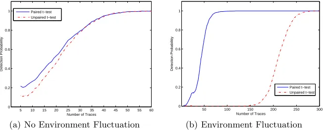
Fig. 5.T-test detection probability for 1O leakage. Again, the paired t-test performs at least as well as the unpaired, while being much more robust in the presence of environmental noise.

With less than 100 pairs, the detection probability of paired t-test is already 1 while unpaired t-test requires much more traces to achieve the same probability. In summary, the paired t-test is more robust and efficient in detecting first order leakage when the power traces are collected in a quickly changing environ-ment.

5.3 Second Order Analysis on a First-Order Resistant Design

In order to validate the effectiveness of the paired t-test in a longer measure-ment campaign, where environmeasure-mental fluctuations are very likely to occur, a first-order-leakage-resistant Simon engine protected by a three-share Threshold Implementation scheme is used as the target. Five million power traces are col-lected in a room without windows and without expected fluctuations in tempera-ture over a period 5 hours. As before, one measurement campaign is performed in a stable lab environment where the environmental conditions are kept as stable as possible. In the other scenario, we again used the hot air blower in intervals of several minutes to simulate stronger environmental noise. This is because the environmental noise might not be strong during the 5-hour collection period. However, in scenarios where hundreds of millions of measurements are needed and taken over a period of several days, then environmental fluctuation can be found, as in Figure 1.

0 1M 2M 3M 4M 5M −1

0 1 2 3 4 5 6 7

Number of Traces

Maximum t value

Unpaired MA−T−test Paired MA−T−test Unpaired T−test Paired T−test

(a) No Environment Fluctuation

0 1M 2M 3M 4M 5M −1

0 1 2 3 4 5 6 7

Number of Traces

Maximum t value

Unpaired MA−T−test Paired MA−T−test Unpaired T−test Paired T−test

(b) Environment Fluctuation

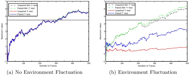
Fig. 6.T-test detection probability for 2O leakage

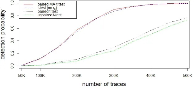
perform about the same with about three million traces needed to achieve a t-statistic above 4.5. This shows that paired t-test works as well as unpaired one for constant collection environment. Also, the moving average based tests perform very similar to the global average based tests, with a minor improvement in the relevant many-traces case. Figure 6(b) depicts the results for the experiment with strong environmental fluctuations. The paired MA-t-test performs best and goes beyond 4.5 faster than the unpaired one. The other two tests using global average are still below the threshold with 5 million traces. The paired t-test still clearly outperforms the unpaired t-test. In sum, the paired t-test based on moving average is the most robust to fluctuation and significantly improves the performance of higher order analysis.

6

Conclusion

Welch’s t-test has recently received a lot of attention as standard side channel security evaluation tool. In this work we showed that noise resulting from envi-ronmental fluctuations can negatively impact the performance of Welch’s t-test. The resulting increased number of observations to detect a leakage are incon-venient and can, in the worst case, result in false conclusions about a device’s resistance. We proposed a paired t-test to improve the standard methodology for leakage detection. The resulting matched-pairs design removes the environ-mental noise effect in leakage detection. Furthermore, we showed that moving averages increase the robustness against environmental noise for higher order or multivariate analysis, while not showing any negative impact in the absence of noise. The improvement is shown through mathematical analysis, simulation, and on practical power measurements: both paired and unpaired t-test with and without the moving averages approach are compared for first order and sec-ond order analysis. Our results show that the proposed (moving average based) paired t-test performed as well or better in all analyzed scenarios. The new method does not increase computational complexity and is numerically more stable than Welch’s t-test. Since our method is more robust to environmental noise and can detect leakage faster than unpaired test in the presence of noise, we propose the replacement of Welch’s t-test with the moving average based paired t-test as a standard leakage detection tool.

Acknowledgments This work is supported by the National Science Foundation under grant CNS-1314655, CNS-1314770 and CNS-1261399 .

References

1. Balasch, J., Gierlichs, B., Grosso, V., Reparaz, O., Standaert, F.X.: On the cost of lazy engineering for masked software implementations. In: Joye, M., Moradi, A. (eds.) Smart Card Research and Advanced Applications, Lecture Notes in Computer Science, vol. 8968, pp. 64–81. Springer International Publishing (2015),

2. Beaulieu, R., Shors, D., Smith, J., Treatman-Clark, S., Weeks, B., Wingers, L.: The simon and speck families of lightweight block ciphers. IACR Cryptology ePrint Archive 2013, 404 (2013)

3. Bilgin, B., Gierlichs, B., Nikova, S., Nikov, V., Rijmen, V.: A More Efficient AES Threshold Implementation. In: Pointcheval, D., Vergnaud, D. (eds.) Progress in Cryptology –AFRICACRYPT 2014, Springer LNCS, vol. 8469, pp. 267–284 (2014) 4. Bilgin, B., Gierlichs, B., Nikova, S., Nikov, V., Rijmen, V.: Higher-order thresh-old implementations. In: Sarkar, P., Iwata, T. (eds.) Advances in Cryptology — ASIACRYPT 2014, Springer LNCS, vol. 8874, pp. 326–343 (2014)

5. Chen, C., Eisenbarth, T., von Maurich, I., Steinwandt, R.: Masking large keys in hardware: A masked implementation of mceliece. In: Selected Areas in Cryptogra-phy - SAC 2015 (2015), (to appear)ia.cr/2015/924

6. Cooper, J., DeMulder, E., Goodwill, G., Jaffe, J., Kenworthy, G., Rohatgi, P.: Test vector leakage assessment (tvla) methodology in practice. In: Inter-national Cryptographic Module Conference (2013), http://icmc-2013.org/wp/ wp-content/uploads/2013/09/goodwillkenworthtestvector.pdf

7. Ding, A., Zhang, L., Fei, Y., Luo, P.: A statistical model for higher order dpa on masked devices. In: Batina, L., Robshaw, M. (eds.) Cryptographic Hardware and Embedded Systems CHES 2014, Lecture Notes in Computer Science, vol. 8731, pp. 147–169. Springer Berlin Heidelberg (2014), http://dx.doi.org/10. 1007/978-3-662-44709-3_9

8. Durvaux, F., Standaert, F.X.: From improved leakage detection to the detection of points of interests in leakage traces. accepted at Eurocrypt 2016 (2016), preprint available athttp://ia.cr/2015/536

9. Goodwill, G., Jun, B., Jaffe, J., Rohatgi, P.: A testing methodol-ogy for side-channel resistance validation. In: NIST Non-Invasive At-tack Testing Workshop (Sept 2011), http://csrc.nist.gov/news_ events/non-invasive-attack-testing-workshop/papers/08_Goodwill.pdf

10. Heuser, A., Kasper, M., Schindler, W., St¨ottinger, M.: A new difference method for side-channel analysis with high-dimensional leakage models. In: Dunkelman, O. (ed.) Topics in Cryptology – CT-RSA 2012, Lecture Notes in Computer Science, vol. 7178, pp. 365–382. Springer Berlin Heidelberg (2012), http://dx.doi.org/ 10.1007/978-3-642-27954-6_23

11. Kutner, M.H., Nachtsheim, C.J., Neter, J., Li, W.: Applied linear statistical models (2005)

12. Leiserson, A.J., Marson, M.E., Wachs, M.A.: Gate-Level Masking under a Path-Based Leakage Metric. In: Batina, L., Robshaw, M. (eds.) Cryptographic Hardware and Embedded Systems – CHES 2014, Springer LNCS, vol. 8731, pp. 580–597 (2014)

13. Mather, L., Oswald, E., Bandenburg, J., W´ojcik, M.: Does my device leak infor-mation? an a priori statistical power analysis of leakage detection tests. In: Sako, K., Sarkar, P. (eds.) Advances in Cryptology - ASIACRYPT 2013, Lecture Notes in Computer Science, vol. 8269, pp. 486–505. Springer Berlin Heidelberg (2013),

http://dx.doi.org/10.1007/978-3-642-42033-7_25

15. Nascimento, E., Lopez, J., Dahab, R.: Efficient and secure elliptic curve cryptog-raphy for 8-bit avr microcontrollers. In: Chakraborty, R.S., Schwabe, P., Solworth, J. (eds.) Security, Privacy, and Applied Cryptography Engineering, Lecture Notes in Computer Science, vol. 9354, pp. 289–309. Springer International Publishing (2015),http://dx.doi.org/10.1007/978-3-319-24126-5_17

16. P´ebay, P.: Formulas for robust, one-pass parallel computation of covariances and arbitrary-order statistical moments. Sandia Report SAND2008-6212, Sandia Na-tional Laboratories (2008)

17. Prouff, E., Rivain, M., Bevan, R.: Statistical analysis of second order differential power analysis. IEEE Trans.on Computers pp. 799 – 811 (2009)

18. Schneider, T., Moradi, A.: Leakage assessment methodology - a clear roadmap for side-channel evaluations. In: Gneysu, T., Handschuh, H. (eds.) CHES. Lecture Notes in Computer Science, vol. 9293, pp. 495–513. Springer (2015),http://dblp. uni-trier.de/db/conf/ches/ches2015.html#SchneiderM15

19. Shahverdi, A., Taha, M., Eisenbarth, T.: Silent simon: A threshold implementation under 100 slices. In: Hardware Oriented Security and Trust (HOST), 2015 IEEE International Symposium on. pp. 1–6 (May 2015)

Appendix

A

Proof of Theorem 1

We are comparing the leakage detection statistic (9)

D= (L(1)_A −L¯(1)_A )(L(2)_A −L¯(2)_A )−(L(1)_B −L¯(1)_B )(L(2)_B −L¯(2)_B ), with the theoretical optimal leakage detection statistic∆in equation (8).

Without loss of generality, let c(1) _{= c}(2) _{= 0 in model (6), since these} constants are cancelled in each of the differences (L(_Aj)−L¯(_Aj)) and (L(_Bj)−L¯(_Bj)) forj= 1,2. Then (8) is simplified as∆=L(1)_A L(2)_A −L(1)_B L(2)_B . Hence

E(∆) =E(L(1)_A L(2)_A )−E(L(1)_B L(2)_B )

V ar(∆) =V ar(L(1)_A L(2)_A ) +V ar(L(1)_B L(2)_B ). (12)

We first reexpress (L(1)_A −L¯(1)_A ) as the difference between two independent terms. We denote ˜L(1)_A = _n1

w−1

Pnw−1

i=1 L

(1)

A,i as the average of nw−1 traces

excluding the original trace, where L(1)_A,i (i = 1, ..., nw −1) are independent

random variables coming from the same distribution as L(1)_A . Since ¯L(1)_A is the average over nw nearby traces including the original trace, ¯L

(1)

A =

1

nw[L

(1)

A +

Pnw−1

i=1 L

(1)

A,i] =

nw−1

nw (L

(1)

A −L˜

(1)

A ), with ˜L

(1)

A independent of L

(1)

A . E( ˜L

(1)

A ) =

E(L(1)_A ) andV ar( ˜L(1)_A ) =_n 1

w−1V ar(L

(1)

A ). Similarly, ˜L

(2)

A , ˜L

(1)

B and ˜L

(2)

B denotes

the average of corresponding quantities over the nw−1 traces excluding the

original trace. The we can rewrite the leakage detection statistic in (9) as

D= (nw−1 nw

Therefore asnw→ ∞,D→∆.

Next, we show that E(D) and V ar(D) differ from their limits E(∆) and V ar(∆) by a factor ofO(1/nw) only. LetD∗=nnww−1D. Then we have

E(D∗) =E(∆), (14)

V ar(D∗)−V ar(∆) = _n2

w[V ar(V

(1)

A )V ar(V

(2)

A ) +V ar(V

(1)

B )V ar(V

(2)

B ) +E

2_(V(1)

A V

(2)

A )

+E2_(V(1)

B V

(2)

B )−V ar(V

(1)

A V

(2)

A )−V ar(V

(1)

B V

(2)

B )] +O(

1

n2

w

).

(15)

The proofs of these two equations are provided in the next two subsections. Combining equations (12), (14) and (15), we arrived at equation (10) and Theorem 1 is proved.

A.1 Proof of Equation (14) on Mean of D∗ We now calculate the first term inE(D).

E( ˜L(1)_A L˜(2)_A ) = ( 1 nw−1

)2

nw−1

X

i=1

nw−1

X

j=1

E(L(1)_A,iL(2)_A,j).

Fori6=j,L(1)_A,iis independence ofL(2)_A,j so thatE(L(1)_A,iL(2)_A,j) =E(L(1)_A,i)E(L(2)_A,j) = (0)(0) = 0 and drops from the summation. Hence

E( ˜L(1)_A L˜(2)_A ) = ( 1 nw−1

)2

nw−1

X

i=1

E(L(1)_A,iL(2)_A,i) = 1 nw−1

E(L(1)_A L(2)_A ). (16)

Also, since ˜L(1)_A is independent of L(2)_A , E( ˜L_A(1)L(2)_A ) = E( ˜L(1)_A )E(L(2)_A ) = 0. SimilarlyE(L(1)_A L˜(2)_A ) = 0. Therefore,

E[(L(1)_A −L˜(1)_A )(L(2)_A −L˜(2)_A )] =E(L(1)_A L(2)_A )−0−0 +E( ˜L(1)_A L˜(2)_A ) =E(L(1)_A L(2)_A ) +_n 1

w−1E(L

(1)

A L

(2)

A )

= nw

nw−1E(L

(1)

A L

(2)

A ).

Similarly, E[(L(1)_B −L˜(1)_B )(L(2)_B −L˜(2)_B )] = nw

nw−1E(L

(1)

B L

(2)

B ).Combine these two

expressions with equation (13) andD∗= nw

nw−1D, we get equation (14)

E(D∗) = (nw−1 nw

) nw nw−1

E[L(1)_A L(2)_A −L(1)_B L(2)_B ] =E(∆).

A.2 Proof of Equation (15) on Variance ofD∗ V ar(D∗) = (nw−1

nw

For the first term, the variance of the sumL(1)_A L(2)_A −L˜(1)_A L_A(2)−L(1)_A L˜(2)_A +L(1)_A L(2)_A is the covariance of the sum with itself. For the four terms inL(1)_A L(2)_A −L˜(1)_A L(2)_A −

L(1)_A L˜(2)_A +L(1)_A L(2)_A , the covariance for most pairs of different terms are zero. For example,

Cov(L(1)_A L(2)_A ,L˜_A(1)L(2)_A ) =E(L(1)_A L(2)_A L˜(1)_A L(2)_A )−E(L(1)_A L(2)_A )E( ˜L(1)_A L(2)_A ) =E(L(1)_A L(2)_A L(2)_A )0−E(L(1)_A L(2)_A )E(L(2)_A )0 = 0.

and Cov(L(1)_A L(2)_A ,L˜(1)_A L˜(2)_A ) = 0 due to the independence betweenL(1)_A L(2)_A and ˜

L(1)_A L˜(2)_A . The only non-zero cross-term covariance is

Cov( ˜L(1)_A L(2)_A , L(1)_A L˜(2)_A ) =E( ˜L(1)_A L(2)_A L(1)_A L˜(2)_A )−0 =E(L(1)_A L(2)_A )E( ˜L(1)_A L˜(2)_A ) =_n 1

w−1E

2_(L(1)

A L

(2)

A ),

with the last step coming from equation (16). Therefore, V ar[(L(1)_A −L˜(1)_A )(L(2)_A −L˜(2)_A )]

=V ar(L(1)_A L(2)_A ) +V ar( ˜L(1)_A L(2)_A ) +V ar(L(1)_A L˜(2)_A ) +V ar( ˜L(1)_A L˜(2)_A )

+ 2

nw−1E

2_(L(1)

A L

(2)

A )

By independence,V ar( ˜L(1)_A L(2)_A ) =V ar( ˜L(1)_A )V ar(L(2)_A ) = _n1

w−1V ar(L

(1)

A )V ar(L

(2)

A ),

andV ar(L(1)_A L˜(2)_A ) =_n 1

w−1V ar(L

(1)

A )V ar(L

(2)

A ).

ForV ar( ˜L(1)_A L˜(2)_A ), note that

˜

L(1)_A L˜(2)_A = ( 1 nw−1

)2

nw−1

X

i=1

nw−1

X

j=1

L(1)_A,iL(2)_A,j.

The covariance between any two different terms in the sum is zero. Hence V ar( ˜L(1)_A L˜(2)_A ) = (_n 1

w−1)

4_[P

iV ar(L

(1)

A,iL

(2)

A,i) +

P

i6=jV ar(L

(1)

A,iL

(2)

A,j)]

=_(n 1

w−1)3V ar(L

(1)

A L

(2)

A ) +

nw−2

(nw−1)3V ar(L

(1)

A )V ar(L

(2)

A ).

Combine together, we have V ar[(L(1)_A −_L˜(1)

A )(L

(2)

A −L˜

(2)

A )]

=V ar(L(1)_A L(2)_A ) + 2

nw−1V ar(L

(1)

A )V ar(L

(2)

A ) +

2

nw−1E

2_(L(1)

A L

(2)

A )

+ nw−2

(nw−1)3V ar(L

(1)

A )V ar(L

(2)

A ) +

1

(nw−1)3V ar(L

(1)

A L

(2)

A )

=V ar(L(1)_A L(2)_A ) +_n2

wV ar(L

(1)

A )V ar(L

(2)

A ) +

2

nwE

2_(L(1)

A L

(2)

A ) +O(

1

n2

w)

Hence the first term inV ar(D∗) becomes (nw−1

nw )

2_{V ar[(L}(1)

A −L˜

(1)

A )(L

(2)

A −L˜

(2)

A )]

= (nw−1

nw )

2_{V ar(L}(1)

A L

(2)

A ) +

2

nwV ar(L

(1)

A )V ar(L

(2)

A ) +

2

nwE

2_(L(1)

A L

(2)

A ) +O(

1

n2

w

) =V ar(L(1)_A L(2)_A ) +_n2

w[V ar(L

(1)

A )V ar(L

(2)

A ) +E

2_(L(1)

A L

(2)

A )−V ar(L

(1)

A L

(2)

A )] +O(

1

n2

w).

For further simplification, letσ2

1 andσ22 denote the variances of noisesr(1) and r(2) _{in the second-order leakage model (6). Then V ar(L}(1)

A ) =σ

2

1+V ar(V(1)), V ar(L(2)_A ) =σ22+V ar(V(2)),E(L

(1)

A L

(2)

A ) =E(V

(1)_V(2)_),

E[(L(1)_A L(2)_A )2_{] =E[(V}(1)

A +r

(1)

A )

2_(V(2)

A +r

(2)

A )

2_] =E[(V_A(1))2_(V(2)

A )

2_{+ (r}(1)

A )

2_(V(2)

A )

2_{+ (V}(1)

A )

2_(r(2)

A )

2_{+ (r}(1)

A )

2_(r(2)

A )

2_{] + 0} =E[(V_A(1))2_(V(2)

A )

2_{] +σ}2 1V ar(V

(2)

A ) +σ

2 2V ar(V

(1)

A ) +σ

2 1σ22. Hence

V ar[L_A(1)L(2)_A ] =V ar(V_A(1)V_A(2)) +σ2₁V ar(V_A(2)) +σ2₂V ar(V_A(1)) +σ₁2σ₂2. Combine the above five expressions,

V ar(L(1)_A )V ar(L(2)_A ) +E2(L(1)_A L(2)_A )−V ar(L(1)_A L(2)_A ) =V ar(V(1))V ar(V(2)) +E(V(1)V(2))−V ar(V_A(1)V_A(2)) Combine this with (17) and (18) we have equation (15),

V ar(D∗)−[V ar(L(1)_A L_A(2)) +V ar(L(1)_B L(2)_B )] = 2

nw[V ar(V

(1)

A )V ar(V

(2)

A ) +E

2_(V(1)

A V

(2)

A )−V ar(V

(1)

A V

(2)

A )

+V ar(V_B(1))V ar(V_B(2)) +E2(V_B(1)V_B(2))−V ar(V_B(1)V_B(2))] +O(_n12

w).

B

Derivation of equation (11)

As in the previous section, we let c(1) _=c(2) _{= 0 without loss of generality, so} that E(L(1)_A ) =E(L(2)_A ) = 0. Then

E[(L(1)_A −b)(L(2)_A −b)] =E(L(1)_A L(2)_A )−bE(L_A(1))−bE(L(2)_A ) +b2=E(L(1)_A L(2)_A ) +b2 =E(L(1)_A L(2)_A ) +b2.

Hence

E(∆∗_b) =E[(L(1)_A −b)(L(2)_A −b)]−E[(L(1)_B −b)(L(2)_B −b)] =E(L(1)_A L(2)_A ) +b2−E(L(1)_B L(2)_B )−b2

=E(L(1)_A L(2)_A )−E(L(1)_B L(2)_B ) =E(∆).

(19)

Next,

V ar[(L(1)_A −b)(L(2)_A −b)] =E[(L(1)_A −b)2_(L(2)

A −b)

2_]−[E(L(1)

A L

(2)

A ) +b

2_]2 =E[((L(1)_A )2_−2bL(1)

A +b

2_)((L(2)

A )

2_−2bL2)

A+b

2_)]−E[(L(1)

A L

(2)

A )

2_]−2bE(L(1)

A L

(2)

A )−b

4

=V ar(L(1)_A L(2)_A )−2bE[L(1)_A L(2)_A (L(1)_A +L(2)_A )] +b2_E[(L(1)

A )

2_{+ (L}(2)

A )

2_{+ 2L}(1)

A L

(2)

A )]

=V ar(L(1)_A L(2)_A ) +b2_{[V ar(L}(1)

A ) +V ar(L

(2)

A ) + 2E(L

(1)

A L

(2)

A )] +O(b).

Hence we get the variance

V ar(∆∗_b) =V ar(∆) +b2_{[V ar(L}(1)

A ) +V ar(L

(2)

A ) + 2E(L

(1)

A L

(2)

A )