MIXED EVOLUTIONARY TECHNIQUES TO REDUCE ORDER OF LINEAR INTERVAL SYSTEMS USING GENERLIZED ROUTH ARRAY

MIXED EVOLUTIONARY

TECHNIQUES TO REDUCE ORDER OF

LINEAR INTERVAL SYSTEMS USING

GENERLIZED ROUTH ARRAY

DEVENDER KUMAR SAINI

Electrical Engineering Deppt. IIT Roorkee, Roorkee, India, Roorkee, Haridwar-247667, India

DR. RAJENDRA PRASAD

Electrical Engineering Deppt. IIT Roorkee, Roorkee, India, Roorkee, Haridwar-247667, India

Abstract:

Recently, genetic algorithms (GA) and particle swarm optimization (PSO) technique have attracted considerable attention among various modern heuristic optimization techniques. In this paper both PSO and GA optimization are employed for finding stable reduced order models of large-scale linear Interval systems. Both the techniques guarantee stability of reduced order model if the original high order model is stable. In both methods interval arithmetic is used to construct generalized Routh array for determining the denominator polynomials of reduced system. The reduced numerator polynomials are determined by minimizing Integral Square Error (ISE) between original and reduced system using GA in first technique and using PSO in second technique pertaining to a unit step input. Both techniques are simple rugged and computer oriented. Both the methods are illustrated through a numerical example and the results are compared with recently published conventional model reduction technique.

Keywords: Interval systems, Interval arithmetic, Genetic Algorithm, Particle Swarm Optimization, Integral Squared Error.

1. Introduction

The exact analysis of high order systems is both tedious and costly as high order systems are too complicated to be used in real problem. Therefore, to analyze such systems, it is necessary to reduce it to a lower order system, which is a sufficient representation of the higher order system. In recent decades, much effort has been made in the field of model reduction for linear dynamic systems and several methods like: Aggregation method [M. Aoki (1968)], Pade approximation [Y. Shamash (1974)], Routh approximation [M.F. Hutton and B. Friendland (1999)], Moment matching technique [N.K. Sinha and B. Kuszta (1983)], Routh-stability technique [V. Krishnamurthy and V. Seshardi (1978)], and ∞ _{optimization technique [K. Glover}

(1984)], have been proposed. Among them Routh stability technique has been recognized as the simplest and powerful method because of its ability to yield stable reduced models for stable high-order systems. Further, numerous methods of order reduction are also available in the literature [Hwang C (1984), Mukherjee S. (1987), Lamba SS (1988), Mukherjee S. (1988), Puri NN (1988), Vilbe P. (1990), Mittal AK. (2004), Howitt GD. (1990)], which are based on minimization of the ISE criterion.

learning mechanism, based loosely on Darwinian principles of biological evolution, reproduction and ‘‘the survival of the fittest’’ [D.E. Goldberg (1989)].

PSO technique was invented in the mid 1990s while attempting to simulate the choreographed, graceful motion of swarms of birds as part of a sociocognative study investigating the notion of collective intelligence in biological populations [J. Kennedy and R.C.Eberhart (1995)].

Both GA and PSO are similar in the sense that these two techniques are population-based search methods and they search for the optimal solution by updating generations. Since the two approaches are supposed to find a solution to a given objective function but employ different strategies and computational effort, it is appropriate to compare their performance.

In general, the practical systems have uncertainties about its parameters. Thus practical systems will have coefficients that may vary and it is represented by interval. Interval arithmetic such as addition, subtraction, multiplication and division are discussed in [E.D. Popova (1994)]. In [B. Bandyopadhyay (1994), B.Bandyopadhyay, A. Upadhye and O.Ismail (1997)] model reduction techniques for higher order uncertain systems were presented using advantage of Routh and Pade approximation methods. The limitations of above method are discussed in [Y. Dolgin and E. Zehab (2003), S.F. Yang (2005)]. A generalized method for constructing the Routh table of interval polynomial is proposed in [Y. Dolgin and E. Zehab (2003)] which overcome some of the limitations of [B. Bandyopadhyay (1994), B.Bandyopadhyay, A. Upadhye and O.Ismail (1997)].

In the present work, the paper present two mixed evolutionary techniques for order reduction of linear interval system based on minimization of the ISE by GA and PSO integrated with modified Routh array for interval systems proposed in [Y. Dolgin and E. Zehab (2003)]. 

2. Reduction Algorithm

Consider a high order linear SISO interval system represented by the transfer function as (1)

, , , ,

, , , , (2)

Where , , 0,1,2, , 1 , , 0,1,2, , are the interval coefficients of higher order numerator and denominator polynomials respectively.

The objective is find a order reduced interval system. Let corresponding order reduced model is

, , , ,

, , , , (3)

Where , , 0,1,2, , 1 , , 0,1,2, , are the interval coefficient of lower order numerator and lower order denominator polynomials respectively.

The rules of the interval arithmetic have been defined as follows. Let [a, b] and [c, d] be two intervals.

Addition:

[a, b]+[c, d] = [a + c, b + d] Subtraction:

[a, b]-[c, d] = [a -d, b - c] Multiplication:

[a, b][c, d] = [Min (ac, ad, bc, bd), Max (ac, ad, bc, bd)] Division:

,

, , , , 0 , .

2.1. Determination of reduced denominator

Dolgin [21]. The reduced denominator is obtained by direct truncation of the elements in the Routh table. Consider the denominator polynomials of higher order system

, , , ,

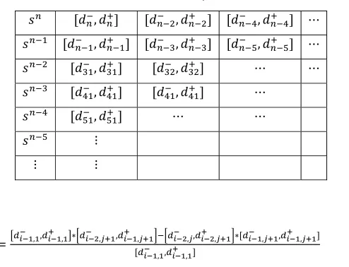
Corresponding generalized Routh table is

Table 1. Generalized Routh array for denominator

, , ,

, , ,

, , , , ,

Where:

,, , , , , ,, , , , ,

,, , (4)

Generalization of the method for direct truncation of Routh table has been proposed in [B. Bandyopadhyay (1994)] for interval systems using interval arithmetic. Based on the fact that a reduced order fixed-coefficients polynomial arrived at by direct truncation of Routh table of a stable higher order polynomial, is guaranteed stable, the authors of [B. Bandyopadhyay (1994)] claim that this is true for interval polynomials as well.

However, in contradiction to what is claimed in [B. Bandyopadhyay (1994)], the property of retaining stability of the reduced polynomial is lost in the interval case, i.e. a stable family of interval polynomials may yield an unstable family of reduced order polynomials arrived at by direct truncation of Routh table using interval arithmetic.

Dolgin (2003) proposed that in order to find coefficients for interval systems use fixed values of ,

and , instead of their intervals. The fixed values may be the midpoints of the intervals or, if desired, the

values which yield the largest intervals for . Order reduced denominator is:

, , , , , , , , ,

, , , 5

2.2. Determination of reduced denominator

The numerator of the reduced order model is determined by minimizing Integral square error between original system and reduced system using genetic algorithm pertaining to a unit step input.

The deviation of the lower order system from the original system response is given by the error index ’ISE’ known as the Integral square error, which is given as follow:

∞

(6)

Where g(t) and r(t) are the unit step response of the original and reduced order systems, respectively.

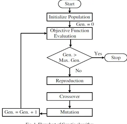
In this method, GA is employed to minimize the objective function ‘ISE’ as given in Eq. (6), and the parameter to be determined are the coefficients of the numerator of the lower order system.

present study are given. The description of GA operators and their properties can be found in [Houck C., Joines J. and Kay M (1995)].

Fig. 1. Flowchart of Genetic algorithm

One more important point that affects the optimal solution more or less is the range for unknowns. For the very first execution of the program, wider solution space can be given and after getting the solution one can shorten the solution space nearer to the values obtained in the previous iteration. The computational flow chart of the proposed algorithm is shown in Fig. 1.

Table 2. Typical Parameters used by Genetic Algorithm

Name Value(type)

Number of generations 200

Population size 100

Type of selection uniform

Type of crossover Arithmetic

Type of mutation uniform

Termination method Maximum generation 2.3.Determination of reduced numerator using PSO

Fig. 2 Description of velocity and position updates in particle swarm optimization for a two dimensional parameter space

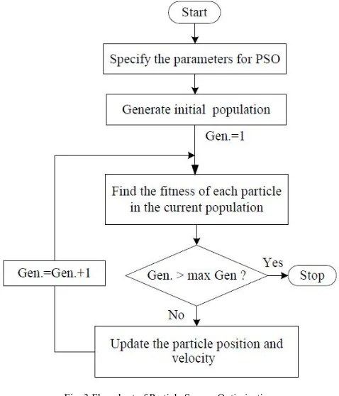
Fig. 3 Flowchart of Particle Swarm Optimization

For the purpose of minimization of Eq. (6), routine from PSO optimization toolbox are used. In Table 3, the typical parameters for PSO optimization routines, used in the present study are given.

Table 3. Typical Parameters used by Particle Swarm Optimization

Name Value(type)

Number of generations 300

Population size 100

Maximum Particle velocity 2

Epoch 100

Termination method Maximum Generation 3. Numerical Example

Where

1.9,2.1 24.7,27.3 157.7,174.3 541.975,599.025 929.955,1027.845 721.81,797.79 187.055,206.745 .

And

. 95,1.05 8.779,9.703 52.231,57.729 182.875,202.125 429.02,474.18 572.47,632.73 325.28,359.52 57.352,63.389

To obtain reduce denominator polynomial, the generalized Routh table is constructed for

Table 4. Generalized Routh array for given example using [Y. Dolgin and E. Zehab (2003)]

. 95,1.05 52.231,57.729 429.02,474.18 325.28,359.52 8.779,9.703 182.875,202.125 572.47,632.73 57.352,63.389 30.36,37.93 360.54,412.2 318.42,353.31

71.34,126.98 476.84,546.54 57.352,63.389 172.37,248.02 296.59,333.56

319.49,406.63 57.352,63.389 259.89,300.36

57.352,63.389

By direct truncation, from above table the second order denominator polynomial is

319.49,406.63 259.89,300.36 57.352,63.389

Thus the 2nd order reduced model using GA becomes

553.9,568.3 181.9,205

And becomes

553.9,568.3 181.9,205

319.49,406.63 259.89,300.36 57.352,63.389

The 2nd _{order model using PSO becomes}

562.4,555.6 181.6,205.4

And becomes

562.4,555.6 181.6,205.4

319.49,406.63 259.89,300.36 57.352,63.389

Following the method of B. Bandyopadhyay (1997) the table for D(s) formed -

[57.35,63.69] [527.47,632.75] [182.88,202.13] [8.78,7.03] [325.28,359.52] [429.02,474.18] [52.23,57.73] [0.95,1.05] [434,623.69] [155.28,214.2] [7.759,10.56] [175.3,564.55] [30.29,77.08] [0.662,1.51] [-36.94,614.78] [0.741,32.37]

The 2nd order system obtained by method [19] is

It is noted that the lower bound of the interval entry , of the table is negative, thus restricting the completion of the table. Hence reduced order interval polynomials of degree four or greater cannot be obtained by [B.Bandyopadhyay (1997)].

4. Results

4.1.Checking Robust Hurwitz Stability of reduced order interval system

Kharitonov (1978) stated that an interval family of polynomials is robustly stable if, and only if, the following Kharitonov polynomials are stable.

_

After Anderson and Jury modified this, they stated that

The testing set for an interval polynomial of invariant degree is

for n=3

, for n=4

, , for n=5

, , , for n 5

For n=1 and n=2, a necessary and sufficient condition for robust stability is positive lower bounds on the coefficients.

The denominator polynomial of the reduced lower order system is

319.49,406.63 259.89,300.36 57.352,63.389

n=2, therefore a necessary and sufficient condition for robust stability is positive lower bounds on the coefficients.

319.49 259.89 57.352

It is clear that is stable. Thus the proposed method guarantees the robust stability of reduced order systems.

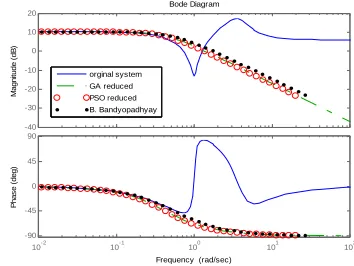
4.2.Simulation Results

Fig. 4 Comparison of step response for lower limit Fig. 5 Comparison of frequency response for lower limit

-60 -40 -20 0 20 Magni tude ( dB )

10-2 10-1 100 101 102 103

-135 -90 -45 0 P has e ( deg) Bode Diagram

Frequency (rad/sec)

orginal system

GA reduced PSO reduced

B. Bandyopadhyay

0 5 10 15 20 25

Fig. 6 Comparison of step response for upper limit Fig. 7 Comparison of frequency response for upper limit

4.3.Comparison of errors

Table 4. Comparison of error for reduced models

Method of

order reduction 2

nd _{Order Reduced Models ISE for lower}

limit ISE for upper limit Proposed GA

Algorithm

. , . . ,

. , . . , . . , . .825 5.562

Proposed PSO Algorithm

. , . . , .

. , . . , . . , . .822 5.558

B. Bandyopadhyay

(1997)

. . . .

. .. . . 2.2599 5.954

5. Conclusion

In this paper, two evolutionary methods for reducing a high order large scale linear interval system into a lower order interval system have been proposed. Particle swarm optimization and genetic algorithm methods based evolutionary optimization techniques are employed for the order reduction where the numerator polynomials are determined by generalized Routh array truncation and denominator coefficients of reduced order model are obtained by minimizing an Integral Squared Error (ISE) criterion.

The proposed method guarantees stability for a stable higher order system and thus any lower order model can be derived with good accuracy. Also it may be noted that the proposed method involves less mathematical complexity compared to algorithm [B.Bandyopadhyay, A. Upadhye and O.Ismail (1997)], where both the γ and δ tables need to be formulated, which increases the complexity and requires a great deal of computational effort. The reduction of seventh order interval system to second order interval system gives excellent step as well as frequency responses. The proposed method is mathematically simple and gives all possible stable lower order models.

References

[1] M. Aoki (1968): Control of large-scale dynamic system by aggregation, IEEE Trans. On Automatic Control, Vol. AC-13, pp. 246-253.

[2] Y. Shamash (1974): Stable reduced order models using Pade type approximations, IEEE trans. On Automatic Control, Vol. 19,

pp.615-616.

[3] M.F. Hutton, B. Friendland (1999): Routh approximations for reducing order of linear time-varying systems, IEEE trans. Automat.

Control, Vol.44, No.9, pp. 1782-1787

[4] N.K. Sinha, B. Kuszta (1983): Modeling and identification of dynamic systems, 133-163, New York: Van Nostrand Reinhold.

[5] V. Krishnamurthy, V. Seshadri (1978): Model Reduction using the Routh Stability Criterion, IEEE Trans. on Automatic Control, Vol.

23 , No. 4.

[6] K. Glover (1984): All optimal Hankel-Norm approximations of linear multivariable systems and their L∞ error bounds, Int. J. Control, Vol. 39, No. 6, pp. 1115-1193.

[7] Hwang C (1984) Mixed method of Routh and ISE criterion approaches for reduced order modeling of continuous time systems. Trans

ASME J Dyn Syst Meas Control 106: 353-356.

[8] Mukherjee S, Mishra RN (1987) Order reduction of linear systems using an error minimization technique. Journal of Franklin Inst

323(1): 23-32. -40 -30 -20 -10 0 10 20 M agn itude ( dB )

10-2 10-1 100 101 102

-90 -45 0 45 90 P has e ( d eg) Bode Diagram

Frequency (rad/sec) orginal system

GA reduced

PSO reduced

B. Bandyopadhyay

0 2 4 6 8 10 12 14 16 18

[9] Lamba SS, Gorez R, Bandyopadhyay B (1988) New reduction technique by step error minimization for multivariable systems. Int. J Systems Sci 19(6): 999-1009.

[10] Mukherjee S, Mishra RN (1988) Reduced order modeling of linear multivariable systems using an error minimization technique.

Journal of Franklin Inst 325(2): 235-245.

[11] Puri NN, Lan DP (1988) Stable model reduction by impulse response error minimization using Mihailov criterion and Pade’s

approximation. Trans ASME J Dyn Syst Meas Control 110: 389-394.

[12] Vilbe P, Calvez LC (1990) On order reduction of linear systems using an error minimization technique. Journal of Franklin Inst 327:

513-514.

[13] Mittal AK, Prasad R, Sharma SP (2004) Reduction of linear dynamic systems using an error minimization technique. Journal of

Institution of Engineers IE (I) Journal – EL 84: 201-206.

[14] Howitt GD, Luus R (1990) Model reduction by minimization of integral square error performance indices. Journal of Franklin Inst

327: 343-357.

[15] D.E. Goldberg (1989), Genetic Algorithms in Search, Optimization, and Machine Learning, Addison-Wesley.

[16] J. Kennedy and R.C.Eberhart (1995), “Particle swarm optimization”, IEEE Int.Conf. on Neural Networks, IV, 1942-1948, Piscataway,

NJ.

[17] E.D. Popova (1994): Extended interval arithmetic in IEEE Floating-Point Environment, Interval Computations, No. 4, pp.

100-129.

[18] Houck C, Joines J, Kay M (1995) A Genetic Algorithm for function optimization: A Matlab implementation. NCSU-IE TR, 95-05.

[19] B. Bandyopadhyay, A. Upadhye, O. Ismail: Routh approximation for interval systems, IEEE Trans. Automat. Control, Vol. 42,

Aug. 1997, pp. 1127– 1130.

[20] B.Bandyopadhyay, et. al. (1994): Routh – Pade approximation for interval systems, IEEE Trans. Automat. Control, Vol. 39, pp.

2454-2456.

[21] Y. Dolgin, E. Zeheb (2003): On Routh-Pade Model Reduction of Interval systems, IEEE Trans. Automat. Control, Vol. 48, pp.

1610-1612.

[22] C. Hwang, S.F. Yang (1999): Comments on the computation of interval Routh approximants, IEEE Trans. Autom. Control, Vol. 44,

No. 9, pp. 1782–1787.

[23] S.F. Yang (2005): Comments on “On Routh–Pade Model Reduction of Interval Systems and Dolgin Y, ’Author’s reply’, IEEE Trans.

Automat. Control, Vol. 50, No. 2, Feb., pp. 273–275.

[24] V.L. Kharitonov (1978): Asymptotic stability of an equilibrium position of a family of systems of linear differential equations,